Performing Inversions of Bolometer Measurements Using Ray Transfer Objects
In this demonstration, we take the geometry matrix and regularisation operator calculated in the Geometry Matrix Calculation Using Ray Transfer Objects demonstration and use them to perform an inversion of simulated bolometer measurements from a defined emissivity profile. The emission source is the same one used in the Defining A Radiation Function demo.
The bolometer system geometry is necessarily the same as that used to calculate the geometry matrix. To perform the inversion we use the regularised NNLS routine, with the voxel grid’s Laplacian operator as the regularisation matrix. The alpha parameter which controls the regularisation was chosen simply by trying different values until the result looked reasonable. Of course, once the measurement vector, geometry matrix and regularisation operator have been calculated then any matrix inversion algorithm can be used to calculate the emissivity profile: we are showcasing one of Cherab’s built-in routines here for convenience.
We have deliberately calculated the measurement vector here by calling the observe
method of BolometerCamera, as this produces measurements independent of the
voxel grid. If many emission profiles are being inverted for the same bolometer and
voxel grid geometries, it would be substantially faster to sample the emission
function on the voxel grid and then multiply this by the sensitivity matrix (this is
done in this demo script to produce the plot of the phantom).
"""
This example demonstrates using a ray transfer object to invert bolometer
measurements and produce a 2D emissivity profile. The bolometer
measurements are provided by observations of a radiating plasma, with
the radiation defined by a 2D function. The inverted emissivity profile
is compared with the original phantom to show the quality of the
inversion.

The bolometer and radiating emitter are produced in the same way as the
`observe_radiation_function.py` demo. We use a simplified cylindrical
geometry and the same radiation function as in the radiation_function.py
demo.
"""
import math
from pathlib import Path
import pickle
import matplotlib.pyplot as plt
import numpy as np

from raysect.core import Node, Point2D, Point3D, Vector3D, rotate_basis, rotate_y, translate
from raysect.optical import World
from raysect.optical.material import AbsorbingSurface, VolumeTransform
from raysect.primitive import Box, Cylinder, Subtract

from cherab.core.math import AxisymmetricMapper, sample2d
from cherab.tools.emitters import RadiationFunction
from cherab.tools.inversions import invert_regularised_nnls
from cherab.tools.observers import BolometerCamera, BolometerSlit, BolometerFoil


# Convenient constants
XAXIS = Vector3D(1, 0, 0)
YAXIS = Vector3D(0, 1, 0)
ZAXIS = Vector3D(0, 0, 1)
ORIGIN = Point3D(0, 0, 0)

# Bolometer geometry: same as the demo which generates the geometry matrix
BOX_WIDTH = 0.05
BOX_WIDTH = 0.2
BOX_HEIGHT = 0.07
BOX_DEPTH = 0.2
SLIT_WIDTH = 0.004
SLIT_HEIGHT = 0.005
FOIL_WIDTH = 0.0013
FOIL_HEIGHT = 0.0038
FOIL_CORNER_CURVATURE = 0.0005
SLIT_SENSOR_SEPARATION = 0.1
FOIL_SEPARATION = 0.00508  # 0.2 inch between foils
SENSOR_ANGLES = [-18, -6, 6, 18]

world = World()


################################################################################
# Make a simple vessel geometry
################################################################################
centre_column_radius = 1
vessel_wall_radius = 3.7
vessel_height = 3.7
vessel = Subtract(
    Cylinder(radius=vessel_wall_radius, height=vessel_height),
    Cylinder(radius=centre_column_radius, height=vessel_height),
    material=AbsorbingSurface(), name="Vessel", parent=world,
)


################################################################################
# Build a simple bolometer system
################################################################################
def make_bolometer_camera():
    # The camera consists of a box with a rectangular slit and 4 sensors, each
    # of which has 4 foils.
    # In its local coordinate system, the camera's slit is located at the
    # origin and the sensors below the z=0 plane, looking up towards the slit.
    camera_box = Box(lower=Point3D(-BOX_WIDTH / 2, -BOX_HEIGHT / 2, -BOX_DEPTH),
                     upper=Point3D(BOX_WIDTH / 2, BOX_HEIGHT / 2, 0))
    # Hollow out the box
    inside_box = Box(lower=camera_box.lower + Vector3D(1e-5, 1e-5, 1e-5),
                     upper=camera_box.upper - Vector3D(1e-5, 1e-5, 1e-5))
    camera_box = Subtract(camera_box, inside_box)
    # The slit is a hole in the box
    aperture = Box(lower=Point3D(-SLIT_WIDTH / 2, -SLIT_HEIGHT / 2, -1e-4),
                   upper=Point3D(SLIT_WIDTH / 2, SLIT_HEIGHT / 2, 1e-4))
    camera_box = Subtract(camera_box, aperture)
    camera_box.material = AbsorbingSurface()
    # Instance of the bolometer camera
    bolometer_camera = BolometerCamera(camera_geometry=camera_box)
    # The bolometer slit in this instance just contains targeting information
    # for the ray tracing, since we have already given our camera a geometry
    # The slit is defined in the local coordinate system of the camera
    slit = BolometerSlit(slit_id="Example slit", centre_point=ORIGIN,
                         basis_x=XAXIS, dx=SLIT_WIDTH, basis_y=YAXIS, dy=SLIT_HEIGHT,
                         parent=bolometer_camera, csg_aperture=False)
    for j, angle in enumerate(SENSOR_ANGLES):
        # 4 bolometer foils, spaced at equal intervals along the local X axis
        # The bolometer positions and orientations are given in the local coordinate
        # system of the camera, just like the slit
        sensor = Node(name="Bolometer sensor", parent=bolometer_camera,
                      transform=rotate_y(angle) * translate(0, 0, -SLIT_SENSOR_SEPARATION))
        # The foils are shifted relative to the centre of the sensor by -1.5, -0.5, 0.5 and 1.5
        # times the foil-foil separation
        for i, shift in enumerate([-1.5, -0.5, 0.5, 1.5]):
            foil_transform = sensor.transform * translate(shift * FOIL_SEPARATION, 0, 0)
            foil = BolometerFoil(detector_id="Foil {} sensor {}".format(i + 1, j + 1),
                                 centre_point=ORIGIN.transform(foil_transform),
                                 basis_x=XAXIS.transform(foil_transform), dx=FOIL_WIDTH,
                                 basis_y=YAXIS.transform(foil_transform), dy=FOIL_HEIGHT,
                                 slit=slit, parent=bolometer_camera, units="Power",
                                 accumulate=False, curvature_radius=FOIL_CORNER_CURVATURE)
            bolometer_camera.add_foil_detector(foil)
    return bolometer_camera


# Make several cameras distributed around the outside of the vessel
camera_angles = [20, 60, 100]
rotation_origin = Point2D(1.5, 1.5)
cameras = []
for camera_angle in camera_angles:
    camera = make_bolometer_camera()
    camera.transform = (translate(rotation_origin.x, 0, rotation_origin.y)
                        * rotate_y(camera_angle)
                        * translate(0, 0, 2.0)
                        * rotate_basis(-ZAXIS, YAXIS)
                        )
    camera.parent = world
    camera.name = "Angle {}".format(camera_angle)
    cameras.append(camera)


################################################################################
# Produce a simple radiating plasma.
################################################################################

# This is the same emission profile used in the radiation_function.py demo,
# but scaled down by 1e6 to make the units on the plots cleaner
PLASMA_AXIS = Point2D(1.5, 1.5)
LCFS_RADIUS = 1
RING_RADIUS = 0.5

RADIATION_PEAK = 1
CENTRE_PEAK_WIDTH = 0.05
RING_WIDTH = 0.025

# distance of wall from LCFS
WALL_LCFS_OFFSET = 0.1

CYLINDER_RADIUS = PLASMA_AXIS.x + LCFS_RADIUS + WALL_LCFS_OFFSET * 1.1
CYLINDER_HEIGHT = (LCFS_RADIUS + WALL_LCFS_OFFSET) * 2


def emission_function_2d(r, z):

    sample_point = Point2D(r, z)
    direction = PLASMA_AXIS.vector_to(sample_point)
    bearing = math.atan2(direction.y, direction.x)

    # calculate radius of coordinate from magnetic axis
    radius_from_axis = direction.length
    closest_ring_point = PLASMA_AXIS + (direction.normalise() * 0.5)
    radius_from_ring = sample_point.distance_to(closest_ring_point)

    # evaluate pedestal-> core function
    if radius_from_axis <= LCFS_RADIUS:

        central_radiatior = RADIATION_PEAK * math.exp(-(radius_from_axis ** 2) / CENTRE_PEAK_WIDTH)

        ring_radiator = (RADIATION_PEAK * math.cos(bearing)
                         * math.exp(-(radius_from_ring ** 2) / RING_WIDTH))
        ring_radiator = max(0, ring_radiator)

        return central_radiatior + ring_radiator
    else:
        return 0


emitter = Cylinder(radius=CYLINDER_RADIUS, height=CYLINDER_HEIGHT,
                   transform=translate(0, 0, 0))
emission_function_3d = AxisymmetricMapper(emission_function_2d)
emitting_material = VolumeTransform(RadiationFunction(emission_function_3d),
                                    transform=emitter.transform.inverse())
emitter.material = emitting_material
emitter.parent = world

################################################################################
# Measure the radiation with the bolometers
################################################################################
print("Measuring the radiation with the bolometers...")
observations = []
for camera in cameras:
    observations.extend(camera.observe())
observations = np.asarray(observations)


################################################################################
# Load the geometry data required for the inversion
################################################################################
script_dir = Path(__file__).parent
try:
    with open(script_dir / "raytransfer_grid_data.pickle", "rb") as f:
        grid_data = pickle.load(f)
except FileNotFoundError:
    raise RuntimeError(
        "Geometry data not found: please run the "
        "geometry_matrix_with_raytransfer.py demo first."
    )

grid_centres = grid_data['grid_centres']
inverse_voxel_map = grid_data['inverse_voxel_map']
grid_laplacian = grid_data['laplacian']
sensitivity_matrix = grid_data['sensitivity_matrix']

# The sensitivity matrix has units of [m3sr].  The radiation function above
# defines an isotropic emissivity with units of [Wm-3], so we need to divide the
# sensitivity matrix by 4pi sr to use with power measurements in [W].
sensitivity_matrix /= 4 * math.pi

################################################################################
# Perform the inversion
################################################################################
print("Performing inversion...")
# We'll use a regularised NNLS inversion here: experience shows it performs
# better than SART for bolometry systems with relatively low numbers of
# foils (though it does perform well for imaging cameras with high resolution).

# Apply a large penalty for placing radiation where there is no bolometer
# coverage, else the algorithm can put radiation there without affecting the
# measurements
grid_laplacian[:, np.nonzero(sensitivity_matrix.sum(axis=0) == 0)] = 1e10

inverted_emission, residual_norm = invert_regularised_nnls(
    sensitivity_matrix, observations, alpha=1e-11, tikhonov_matrix=grid_laplacian
)

################################################################################
# Plot the emissivity profile and the inverted profile
################################################################################
print("Plotting results...")
# Sample the phantom emission to produce a 2D plot
rsampled, zsampled, phantom_samples = sample2d(
    emission_function_2d,
    (grid_centres.take(0, -1).min(), grid_centres.take(0, -1).max(), grid_centres.shape[0]),
    (grid_centres.take(1, -1).min(), grid_centres.take(1, -1).max(), grid_centres.shape[1]),
)

# Convert the 1D emissivity vector from the inversion into a 2D array
# This method is general enough to handle an arbitrary voxel map, with different
# numbers of grid cells inside each voxel (although we don't need it here). See
# the geometry_matrix_with_raytransfer.py demo for a shorter, faster method using
# the grid mask when there is a 1-to-1 mapping of grid cells to voxels.

# Just like in the geometry_matrix_with_raytransfer.py demo, we are storing
# axisymmetric data in 2D arrays but the ray transfer objects are fully
# 3D. Therefore we need to pad our data to 3D views when using indices
# provided by the ray transfer objects.
inversion_2d = np.full_like(phantom_samples, np.nan)
for indices, emission in zip(inverse_voxel_map, inverted_emission):
    inversion_2d[:, None, :][tuple(np.squeeze(indices).T)] = emission
# Note that cells not part of any voxel contain nan: they are undefined in the
# inversion. This has the nice side effect that they show up without a colour in
# the plot.

fig, (ax1, ax2) = plt.subplots(1, 2)
phantom_image = ax1.imshow(
    phantom_samples.T, interpolation="none", origin="lower",
    extent=(rsampled.min(), rsampled.max(), zsampled.min(), zsampled.max())
)
fig.colorbar(phantom_image, ax=ax1)
ax1.set_title("Phantom")
ax1.set_xlabel("r")
ax1.set_ylabel("z")
inversion_image = ax2.imshow(
    inversion_2d.T, interpolation="none", origin="lower",
    extent=(rsampled.min(), rsampled.max(), zsampled.min(), zsampled.max())
)
fig.colorbar(inversion_image, ax=ax2)
ax2.set_title("Inversion")
ax2.set_xlabel("r")
ax2.set_ylabel("z")
fig.tight_layout()

################################################################################
# Calculate some metrics for comparison with the phantom
################################################################################
back_calculated_measurements = sensitivity_matrix @ inverted_emission
voxel_phantom_samples = np.asarray([phantom_samples[:, None, :][voxel].sum()
                                    for voxel in inverse_voxel_map])
phantom_measurements = sensitivity_matrix @ voxel_phantom_samples
cell_dx = grid_centres[1, 0, 0] - grid_centres[0, 0, 0]
cell_dy = grid_centres[0, 1, 1] - grid_centres[0, 0, 1]
voxel_rs = grid_centres.take(0, -1)
voxel_volumes = np.asarray([(2 * np.pi * voxel_rs[:, None, :][voxel] * cell_dx * cell_dy).sum()
                            for voxel in inverse_voxel_map])
total_phantom_power = voxel_phantom_samples @ voxel_volumes
total_inversion_power = inverted_emission @ voxel_volumes

fig, ax = plt.subplots()
ax.plot(observations, linestyle="-", label="Ray-traced measurements")
ax.plot(phantom_measurements, linestyle="--", label="Raytransfer-based measurements")
ax.plot(back_calculated_measurements, linestyle="--", label="Back-calculated from inversion")
ax.set_xlabel("Foil")
ax.set_ylabel("Power / W")
ax.legend()

print("Phantom total power: {:.4g}W".format(total_phantom_power))
print("Inversion total power: {:.4g}W".format(total_inversion_power))

plt.show()
The demo prints the total power calculated from the phantom emissivity profile and the inverted profile. There is good agreement between the two, with only a 5% discrepancy.
Measuring the radiation with the bolometers...
Performing inversion...
Plotting results...
Phantom total power: 4.848W
Inversion total power: 5.13W
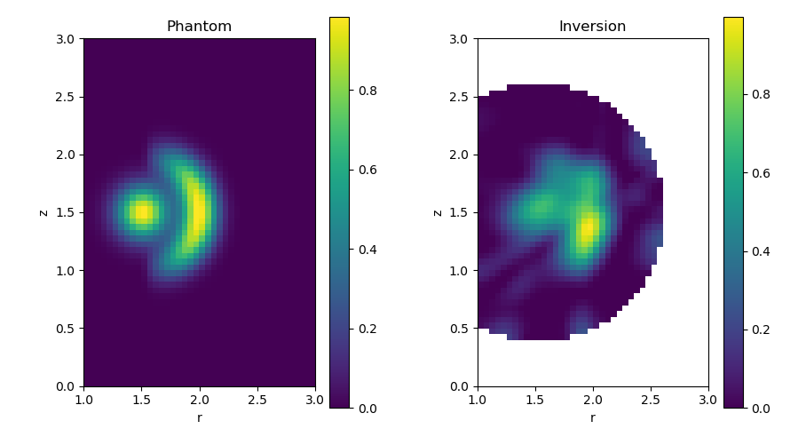
Caption The input and reconstructed emissivity profiles. The general profile shape is preserved, with the central blob and ring radiator visible in the inversion. There are a few artefacts around the edge of the reconstruction volume, Note also that there is more blurring of the boundary between the central and ring radiators in the upper half of the image: this reflects the fact that the bolometer sightlines are not symmetric above and below the midplane.

Caption The forward-modelled and back-calculated power measurements on the foils. The measured power using ray tracing in this script, the calculated power by multiplying the sensitivity matrix by the emission vector and the back-calculated power calculated by multiplying the sensitivity matrix by the inverted emissivity are all in good agreement, showing that the grid size and the amount of regularisation are suitable in this case.