Defining A Radiation Function
When calculating surface radiation loads on reactor components it is necessary to define a radiation function. This could be some output from a physics code, or perhaps an analytic function. In Cherab, the source function will always be prescribed as a 3D function regardless of the data source.
All emission models in Cherab and Raysect are fully spectral. It is possible to
create arbitrary radiation functions using the Material interface in Raysect.
However it is often sufficient to specify a simple total radiated power
function in terms of W/m^2 for many physics applications. In such cases, the
RadiationFunction utility
material is particularly useful.
In this example we give it a user specified python function that specifies the emission, and attach it to a cylinder. The surface of the cylinder is transparent, but its volume emits proportional to the specified function. Note that the radiation function is evaluated in the local coordinate system of the primitive to which the material is attached. In this example we create a cylinder which is shifted in the Z direction, but we want to evaluate the radiation function in the unshifted “global” coordinate system. For this we can use raysect’s VolumeMaterial material modifier.
import numpy as np
import matplotlib.pyplot as plt

from raysect.core import Point2D, translate, Vector3D, rotate_basis
from raysect.primitive import Cylinder
from raysect.optical import World
from raysect.optical.observer import PinholeCamera, PowerPipeline2D
from raysect.optical.material import VolumeTransform

from cherab.core.math import sample2d, AxisymmetricMapper
from cherab.tools.emitters import RadiationFunction


#############################
# define radiation function #


PLASMA_AXIS = Point2D(1.5, 0)
LCFS_RADIUS = 1
RING_RADIUS = 0.5

RADIATION_PEAK = 1e6
CENTRE_PEAK_WIDTH = 0.05
RING_WIDTH = 0.025

# distance of wall from LCFS
WALL_LCFS_OFFSET = 0.1

CYLINDER_RADIUS = PLASMA_AXIS.x + LCFS_RADIUS + WALL_LCFS_OFFSET * 1.1
CYLINDER_HEIGHT = (LCFS_RADIUS + WALL_LCFS_OFFSET) * 2


def rad_function(r, z):

    sample_point = Point2D(r, z)
    direction = PLASMA_AXIS.vector_to(sample_point)
    bearing = np.arctan2(direction.y, direction.x)

    # calculate radius of coordinate from magnetic axis
    radius_from_axis = direction.length
    closest_ring_point = PLASMA_AXIS + (direction.normalise() * 0.5)
    radius_from_ring = sample_point.distance_to(closest_ring_point)

    # evaluate pedestal-> core function
    if radius_from_axis <= LCFS_RADIUS:

        central_radiatior = RADIATION_PEAK * np.exp(-(radius_from_axis ** 2) / CENTRE_PEAK_WIDTH)

        ring_radiator = RADIATION_PEAK * np.cos(bearing) * np.exp(-(radius_from_ring ** 2) / RING_WIDTH)
        ring_radiator = max(0, ring_radiator)

        return central_radiatior + ring_radiator
    else:
        return 0


#################################
# add radiation source to world #

world = World()

rad_function_3d = AxisymmetricMapper(rad_function)
# We shift the cylinder containing the emission function relative to the world,
# so need to apply the opposite shift to the material to ensure the radiation
# function is evaluated in the correct coordinate system.
shift = translate(0, 0, -1)
radiation_emitter = VolumeTransform(RadiationFunction(rad_function_3d), shift.inverse())
geom = Cylinder(CYLINDER_RADIUS, CYLINDER_HEIGHT,
                transform=shift, parent=world, material=radiation_emitter)


######################
# visualise emission #

# run some plots to check the distribution functions and emission profile are as expected
r, z, t_samples = sample2d(rad_function, (0, 4, 200), (-2, 2, 200))
plt.imshow(np.transpose(np.squeeze(t_samples)), extent=[0, 3, -1.5, 1.5])
plt.colorbar()
plt.axis('equal')
plt.xlabel('r axis')
plt.ylabel('z axis')
plt.title("Radiation profile in r-z plane")


camera = PinholeCamera((256, 256), pipelines=[PowerPipeline2D()], parent=world)
camera.transform = translate(-3.5, -1.5, 0)*rotate_basis(Vector3D(1, 0, 0), Vector3D(0, 0, 1))
camera.pixel_samples = 1

plt.ion()
camera.observe()
plt.ioff()
plt.show()
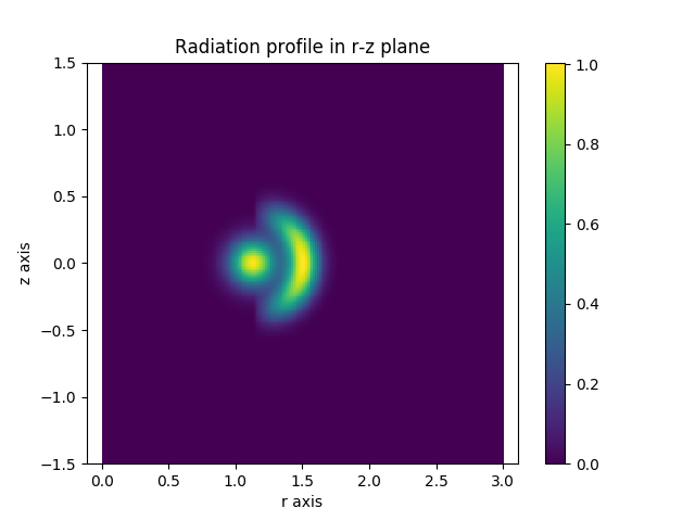
Caption: A slice through the specified 3D emission function in the R-Z plane..
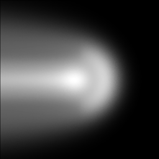
Caption: A camera visualiation of the emission function. Notice that the bounding cylinder is transparent so there are effectively no walls. The emission function is defined inside the bounding cylinder and zero everywhere else.