Calculating a Geometry Matrix using Ray Transfer Objects
In this demonstration, we calculate the geometry matrix for a slightly more complicated bolometer system, consisting of 3 cameras each of which have 16 foils looking through a single aperture. This produces the same end result as the Geometry Matrix With Voxels demo, but with significantly higher performance when calculating the sensitivity matrix itself. Since the voxel demo uses axisymmetric voxels with a rectangular cross section the results of the two frameworks are directly comparable. Voxels with arbitrary gometry cannot be represented exactly with the ray transfer framework, but can be approximated by combining multiple cubiod or axisymmetic (with rectangular cross section) cells into single larger voxels. With a large enough number of cells the approximation will be quite good.
In addition to the geometry matrix, a regularisation operator is generated. This is needed for regularised tomographic inversions, as shown in the Inversion with Ray Transfer Objects demo. We use a simple Laplacian operator as the regularisation operator, which corresponds to isotropic smoothing.
"""
This example demonstrates calculating the geometry matrix for a
bolometer system using ray transfer matrices. The discretisation grid is
the same as that used in the corresponding voxel example, but the ray
transfer objects have better performance than voxels as the expense of
pixellated cells.
"""
import math
from pathlib import Path
import pickle
import matplotlib.pyplot as plt
from matplotlib.patches import Rectangle
import numpy as np

from raysect.core import Node, Point2D, Point3D, Vector3D, rotate_basis, rotate_y, translate
from raysect.optical import World
from raysect.optical.material import AbsorbingSurface
from raysect.primitive import Box, Cylinder, Subtract

from cherab.tools.raytransfer import RayTransferCylinder, RayTransferPipeline0D
from cherab.tools.observers import BolometerCamera, BolometerSlit, BolometerFoil


# Convenient constants
XAXIS = Vector3D(1, 0, 0)
YAXIS = Vector3D(0, 1, 0)
ZAXIS = Vector3D(0, 0, 1)
ORIGIN = Point3D(0, 0, 0)
# Bolometer geometry
BOX_WIDTH = 0.05
BOX_WIDTH = 0.2
BOX_HEIGHT = 0.07
BOX_DEPTH = 0.2
SLIT_WIDTH = 0.004
SLIT_HEIGHT = 0.005
FOIL_WIDTH = 0.0013
FOIL_HEIGHT = 0.0038
FOIL_CORNER_CURVATURE = 0.0005
SLIT_SENSOR_SEPARATION = 0.1
FOIL_SEPARATION = 0.00508  # 0.2 inch between foils
SENSOR_ANGLES = [-18, -6, 6, 18]

world = World()


########################################################################
# Make a simple vessel geometry
########################################################################
centre_column_radius = 1
vessel_wall_radius = 3.7
vessel_height = 3.7
vessel = Subtract(
    Cylinder(radius=vessel_wall_radius, height=vessel_height),
    Cylinder(radius=centre_column_radius, height=vessel_height),
    material=AbsorbingSurface(), name="Vessel", parent=world,
)


########################################################################
# Build a simple bolometer system
########################################################################
def make_bolometer_camera():
    # The camera consists of a box with a rectangular slit and 4 sensors,
    # each of which has 4 foils.
    # In its local coordinate system, the camera's slit is located at the
    # origin and the sensors below the z=0 plane, looking up towards the slit.
    camera_box = Box(lower=Point3D(-BOX_WIDTH / 2, -BOX_HEIGHT / 2, -BOX_DEPTH),
                     upper=Point3D(BOX_WIDTH / 2, BOX_HEIGHT / 2, 0))
    # Hollow out the box
    inside_box = Box(lower=camera_box.lower + Vector3D(1e-5, 1e-5, 1e-5),
                     upper=camera_box.upper - Vector3D(1e-5, 1e-5, 1e-5))
    camera_box = Subtract(camera_box, inside_box)
    # The slit is a hole in the box
    aperture = Box(lower=Point3D(-SLIT_WIDTH / 2, -SLIT_HEIGHT / 2, -1e-4),
                   upper=Point3D(SLIT_WIDTH / 2, SLIT_HEIGHT / 2, 1e-4))
    camera_box = Subtract(camera_box, aperture)
    camera_box.material = AbsorbingSurface()
    # Instance of the bolometer camera
    bolometer_camera = BolometerCamera(camera_geometry=camera_box)
    # The bolometer slit in this instance just contains targeting information
    # for the ray tracing, since we have already given our camera a geometry
    # The slit is defined in the local coordinate system of the camera
    slit = BolometerSlit(slit_id="Example slit", centre_point=ORIGIN,
                         basis_x=XAXIS, dx=SLIT_WIDTH, basis_y=YAXIS, dy=SLIT_HEIGHT,
                         parent=bolometer_camera)
    for j, angle in enumerate(SENSOR_ANGLES):
        # 4 bolometer foils, spaced at equal intervals along the local X axis
        # The bolometer positions and orientations are given in the local coordinate
        # system of the camera, just like the slit
        sensor = Node(name="Bolometer sensor", parent=bolometer_camera,
                      transform=rotate_y(angle) * translate(0, 0, -SLIT_SENSOR_SEPARATION))
        # The foils are shifted relative to the centre of the sensor by -1.5, -0.5, 0.5 and 1.5
        # times the foil-foil separation
        for i, shift in enumerate([-1.5, -0.5, 0.5, 1.5]):
            # Note that the foils will be parented to the camera rather than the
            # sensor, so we need to define their transform relative to the camera
            foil_transform = sensor.transform * translate(shift * FOIL_SEPARATION, 0, 0)
            foil = BolometerFoil(detector_id="Foil {} sensor {}".format(i + 1, j + 1),
                                 centre_point=ORIGIN.transform(foil_transform),
                                 basis_x=XAXIS.transform(foil_transform), dx=FOIL_WIDTH,
                                 basis_y=YAXIS.transform(foil_transform), dy=FOIL_HEIGHT,
                                 slit=slit, parent=bolometer_camera, units="Power",
                                 accumulate=False, curvature_radius=FOIL_CORNER_CURVATURE)
            bolometer_camera.add_foil_detector(foil)
    return bolometer_camera


# Make several cameras distributed around the outside of the vessel
camera_angles = [20, 60, 100]
rotation_origin = Point2D(1.5, 1.5)
cameras = []
for camera_angle in camera_angles:
    camera = make_bolometer_camera()
    camera.transform = (translate(rotation_origin.x, 0, rotation_origin.y)
                        * rotate_y(camera_angle)
                        * translate(0, 0, 2.0)
                        * rotate_basis(-ZAXIS, YAXIS)
                        )
    camera.parent = world
    camera.name = "Angle {}".format(camera_angle)
    cameras.append(camera)


########################################################################
# Show the lines of sight of all the bolometer channels
########################################################################
def _point3d_to_rz(point):
    return Point2D(math.hypot(point.x, point.y), point.z)


fig, ax = plt.subplots()
all_foils = [foil for camera in cameras for foil in camera]
for foil in all_foils:
    slit_centre = foil.slit.centre_point
    slit_centre_rz = _point3d_to_rz(slit_centre)
    ax.plot(slit_centre_rz[0], slit_centre_rz[1], 'ko')
    origin, hit, _ = foil.trace_sightline()
    centre_rz = _point3d_to_rz(foil.centre_point)
    ax.plot(centre_rz[0], centre_rz[1], 'kx')
    origin_rz = _point3d_to_rz(origin)
    hit_rz = _point3d_to_rz(hit)
    ax.plot([origin_rz[0], hit_rz[0]], [origin_rz[1], hit_rz[1]], 'k')

ax.add_patch(Rectangle((centre_column_radius, 0), edgecolor='k', facecolor='none',
                       width=(vessel_wall_radius - centre_column_radius),
                       height=vessel_height,))
ax.axis('equal')
ax.set_title("Bolometer camera lines of sight")
ax.set_xlabel("r")
ax.set_ylabel("z")

########################################################################
# Produce a voxel grid
########################################################################
print("Producing the voxel grid...")
# Define the centres of each voxel, as an (nx, ny, 2) array
nx = 40
ny = 60
cell_r, cell_dx = np.linspace(1, 3, nx, retstep=True)
cell_z, cell_dz = np.linspace(0, 3, ny, retstep=True)
cell_r_grid, cell_z_grid = np.broadcast_arrays(cell_r[:, None], cell_z[None, :])
cell_centres = np.stack((cell_r_grid, cell_z_grid), axis=-1)  # (nx, ny, 2) array

# Define the positions of the vertices of the voxels
cell_vertices_r = np.linspace(cell_r[0] - 0.5 * cell_dx, cell_r[-1] + 0.5 * cell_dx, nx + 1)
cell_vertices_z = np.linspace(cell_z[0] - 0.5 * cell_dz, cell_z[-1] + 0.5 * cell_dz, ny + 1)

# Build a mask, only including cells within the wall
# The inversions will be performed on the emission profile used in the
# radiation_function.py demo, so we'll trim the voxel grid down to the
# emitting region
PLASMA_AXIS = Point2D(1.5, 1.5)
LCFS_RADIUS = 1
WALL_LCFS_OFFSET = 0.1  # distance of the virtual inner wall from LCFS

vertex_radius_squared = ((cell_vertices_r[:, None] - PLASMA_AXIS.x)**2
                         + (cell_vertices_z[None, :] - PLASMA_AXIS.y)**2)
vertex_mask = vertex_radius_squared <= (WALL_LCFS_OFFSET + LCFS_RADIUS)**2
# Cell is included if at least one vertex is within the wall
grid_mask = (vertex_mask[1:, :-1] + vertex_mask[:-1, :-1]
             + vertex_mask[1:, 1:] + vertex_mask[:-1, 1:])
# The RayTransferCylinder object is fully 3D, but for simplicity we're only
# working in 2D as this case is axisymmetric. It is easy enough to pass 3D
# views of our 2D data into the RayTransferCylinder object: we just ues a
# numpy.newaxis (or equivalently, None) for the toroidal dimension.
grid_mask = grid_mask[:, None, :]

num_cells = grid_mask.sum()

ray_transfer_grid = RayTransferCylinder(
    radius_outer=cell_vertices_r[-1],
    radius_inner=cell_vertices_r[0],
    height=cell_vertices_z[-1] - cell_vertices_z[0],
    n_radius=nx, n_height=ny, mask=grid_mask, n_polar=1,
    transform=translate(0, 0, cell_vertices_z[0])
)

########################################################################
# Produce a regularisation operator for inversions
########################################################################
# We'll use simple isotropic smoothing here, in which case an ND second
# derivative operator (the laplacian operator) is appropriate. This can be
# produced in the same way as in the geometry matrix with voxels demo, but we
# show a faster vectorised method here.

# Pad the voxel map with a 1-cell-wide border.
voxel_map_with_borders = - np.ones((nx + 2, ny + 2), dtype=int)
voxel_map_with_borders[1:-1, 1:-1] = ray_transfer_grid.voxel_map[:, 0, :]
inverted_voxel_map = ray_transfer_grid.invert_voxel_map()
grid_laplacian = np.zeros((num_cells, num_cells))


for ith_cell in range(num_cells):

    # get the 2D mesh coordinates of this cell
    ix, _, iy = inverted_voxel_map[ith_cell]
    # we didn't map multiple cells into the same light source,
    # so ix and iy are single-element arrays
    ix = ix[0]
    iy = iy[0]

    neighbours_2d = ([ix, ix, ix, ix + 1, ix + 1, ix + 2, ix + 2, ix + 2],
                     [iy, iy + 1, iy + 2, iy, iy + 2, iy, iy + 1, iy + 2])

    neighbours_1d = voxel_map_with_borders[neighbours_2d]
    neighbours_1d = neighbours_1d[neighbours_1d > -1]

    grid_laplacian[ith_cell, neighbours_1d] = -1
    grid_laplacian[ith_cell, ith_cell] = neighbours_1d.size


########################################################################
# Calculate the geometry matrix for the grid
########################################################################
print("Calculating the geometry matrix...")
# The ray transfer object must be in the same world as the bolometers
ray_transfer_grid.parent = world

sensitivity_matrix = []
for camera in cameras:
    for foil in camera:
        print("Calculating sensitivity for {}...".format(foil.name))
        foil.pipelines = [RayTransferPipeline0D(kind=foil.units)]
        # All objects in world have wavelength-independent material properties,
        # so it doesn't matter which wavelength range we use (as long as
        # max_wavelength - min_wavelength = 1)
        foil.min_wavelength = 1
        foil.max_wavelength = 2
        foil.spectral_bins = ray_transfer_grid.bins
        foil.observe()
        sensitivity_matrix.append(foil.pipelines[0].matrix)
sensitivity_matrix = np.asarray(sensitivity_matrix)

# Plot the sensitivity matrix, summed over all foils
# We used a mask to construct the ray transfer grid, so have a 1-to-1 mapping of
# grid cells to voxels. We can thus use the mask the map the voxel data back to
# the 2D grid. A more general method which works if multiple cells are mapped to
# a single voxel can be seen in the inversion_with_raytransfer.py demo.
sensitivity_2d = np.full((nx, ny), np.nan)
sensitivity_2d[ray_transfer_grid.mask[:, 0, :]] = sensitivity_matrix.sum(axis=0)

fig, ax = plt.subplots()
image = ax.imshow(sensitivity_2d.T, origin="lower", interpolation="none",
                  extent=(cell_r.min(), cell_r.max(), cell_z.min(), cell_z.max()))
fig.colorbar(image)
ax.set_title("Total sensitivity [m³sr]")
ax.set_xlabel("r")
ax.set_ylabel("z")

# Save the voxel grid information and the geometry matrix for use in other demos
ray_transfer_grid_data = {
    'grid_centres': cell_centres,
    'voxel_map': ray_transfer_grid.voxel_map,
    'inverse_voxel_map': ray_transfer_grid.invert_voxel_map(),
    'laplacian': grid_laplacian,
    'mask': ray_transfer_grid.mask,
    'sensitivity_matrix': sensitivity_matrix
}

script_dir = Path(__file__).parent
with open(script_dir / "raytransfer_grid_data.pickle", "wb") as f:
    pickle.dump(ray_transfer_grid_data, f)

plt.show()

Caption The lines of sight of the 48 foils in 3 bolometer cameras, used to generate the sensitivity matrix.
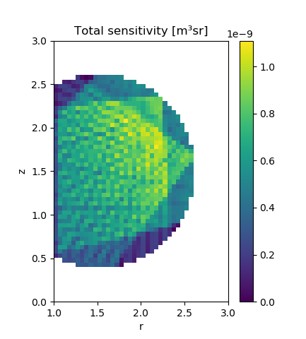
Caption The result of summing the sensitivty of all foils, for each voxel in the ray transfer object. Since we are using a mask, only a subset of the ray transfer object’s cells are treated as voxels to be calculated: in the rest the sensitivity is undefined.