Symmetric Power Load Calculation

In this example we perform a simple radiation load calculation by exploiting symmetry, building on the previous examples. We use an analytic radiation function combined with a simple toroidal wall. The actual wall detectors are constructed manually using the Raysect Pixel detector class.

Note

Observing surface are transparent in Raysect. Rays are launched from these surfaces, but Ray’s don’t collide with them. If you want them to act as absorbers you need to separately add an absorbing surface. To avoid numerical issues, its important that these surfaces are slightly displaced. If they overlap, some rays will become trapped within the surface due to numerical rounding, leading to faulty calculations. Its best to separate these surfaces with some small numerical scale length.

import numpy as np
import matplotlib.pyplot as plt

from raysect.core import Point2D, Point3D, translate, Vector3D, rotate_basis
from raysect.optical import World, Spectrum
from raysect.primitive import Cylinder
from raysect.optical.observer import PowerPipeline0D
from raysect.optical.observer.nonimaging.pixel import Pixel
from raysect.optical.material import AbsorbingSurface, VolumeTransform

from cherab.core.math import sample2d, AxisymmetricMapper
from cherab.tools.emitters import RadiationFunction
from cherab.tools.primitives import axisymmetric_mesh_from_polygon


#############################
# define radiation function #

PLASMA_AXIS = Point2D(1.5, 0)
PLASMA_AXIS_3D = Point3D(PLASMA_AXIS.x, 0.0, PLASMA_AXIS.y)  # convert the plasma_axis in a 3D point
LCFS_RADIUS = 1
RING_RADIUS = 0.5

RADIATION_PEAK = 1e6
CENTRE_PEAK_WIDTH = 0.05
RING_WIDTH = 0.025

# distance of wall from LCFS
WALL_LCFS_OFFSET = 0.1

# distance of detector pixels from wall
# slightly displaced to avoid numerical overlap (ray trapping)
WALL_DETECTOR_OFFSET = 0.001

CYLINDER_RADIUS = PLASMA_AXIS.x + LCFS_RADIUS + WALL_LCFS_OFFSET * 1.1
CYLINDER_HEIGHT = (LCFS_RADIUS + WALL_LCFS_OFFSET) * 2
WALL_RADIUS = LCFS_RADIUS + WALL_LCFS_OFFSET
DETECTOR_RADIUS = WALL_RADIUS - WALL_DETECTOR_OFFSET


def rad_function(r, z):

    sample_point = Point2D(r, z)
    direction = PLASMA_AXIS.vector_to(sample_point)
    bearing = np.arctan2(direction.y, direction.x)

    # calculate radius of coordinate from magnetic axis
    radius_from_axis = direction.length
    closest_ring_point = PLASMA_AXIS + (direction.normalise() * 0.5)
    radius_from_ring = sample_point.distance_to(closest_ring_point)

    # evaluate pedestal-> core function
    if radius_from_axis <= LCFS_RADIUS:

        central_radiatior = RADIATION_PEAK * np.exp(-(radius_from_axis ** 2) / CENTRE_PEAK_WIDTH)

        ring_radiator = RADIATION_PEAK * np.cos(bearing) * np.exp(-(radius_from_ring ** 2) / RING_WIDTH)
        ring_radiator = max(0, ring_radiator)

        return central_radiatior + ring_radiator
    else:
        return 0


# add radiation source to world
shift = translate(0, 0, -1)
rad_function_3d = AxisymmetricMapper(rad_function)
radiation_emitter = VolumeTransform(RadiationFunction(rad_function_3d), shift.inverse())

world = World()
geom = Cylinder(CYLINDER_RADIUS, CYLINDER_HEIGHT,
                transform=shift, parent=world, material=radiation_emitter)


############################################
# make a toroidal wall wrapping the plasma #

# number of poloidal wall elements
n_poloidal = 250
d_angle = (2*np.pi) / n_poloidal

wall_polygon = np.zeros((n_poloidal, 2))
for i in range(n_poloidal):
    pr = PLASMA_AXIS.x + WALL_RADIUS * np.sin(d_angle * i)
    pz = PLASMA_AXIS.y + WALL_RADIUS * np.cos(d_angle * i)
    wall_polygon[i, :] = pr, pz
wall_polygon = wall_polygon[::-1]  # make surface normals point inwards

# create a 3D mesh from the 2D polygon outline using symmetry
wall_mesh = axisymmetric_mesh_from_polygon(wall_polygon)
wall_mesh.parent = world
wall_mesh.material = AbsorbingSurface()


###################################################
# make detectors wrapping a slice of wall surface #

# toroidal width of the detectors
X_WIDTH = 0.01

# intialization of the initial angle
d_angle = (2*np.pi) / n_poloidal

# visualise emission adn detectors
plt.figure()
r, z, t_samples = sample2d(rad_function, (0, 4, 200), (-2, 2, 200))
plt.imshow(np.transpose(np.squeeze(t_samples)), extent=[0, 4, -2, 2])
plt.colorbar()
plt.axis('equal')
plt.xlabel('r axis')
plt.ylabel('z axis')
plt.title("Radiation profile in r-z plane")

wall_detectors = []
for index in range(1, n_poloidal + 1):

    p1x = PLASMA_AXIS.x + DETECTOR_RADIUS * np.sin(d_angle * index)
    p1y = PLASMA_AXIS.y + DETECTOR_RADIUS * np.cos(d_angle * index)
    p1 = Point3D(p1x, 0, p1y)

    p2x = PLASMA_AXIS.x + DETECTOR_RADIUS * np.sin(d_angle * (index + 1))
    p2y = PLASMA_AXIS.y + DETECTOR_RADIUS * np.cos(d_angle * (index + 1))
    p2 = Point3D(p2x, 0, p2y)

    # evaluate y_vector
    y_vector_full = p1.vector_to(p2)
    y_vector = y_vector_full.normalise()
    y_width = y_vector_full.length

    # evaluate the central point of the detector
    detector_center = p1 + y_vector_full * 0.5

    # evaluate normal_vector
    normal_vector = (detector_center.vector_to(PLASMA_AXIS_3D)).normalise()  # inward pointing

    # to populate it step by step
    wall_detectors = wall_detectors + [((index - 1), X_WIDTH, y_width, detector_center, normal_vector, y_vector)]

    plt.plot([p1x, p2x], [p1y, p2y], 'k')
    plt.plot([p1x, p2x], [p1y, p2y], '.k')
    pc = detector_center
    pcn = pc + normal_vector * 0.05
    plt.plot([pc.x, pcn.x], [pc.z, pcn.z], 'r')


##############################################################
# iterate through all detectors and calculate radiation load #

# storage lists for results
power_densities = []
detector_numbers = []
distance = []

running_distance = 0
observed_total_power = 0

# loop over each tile detector
for i, detector in enumerate(wall_detectors):

    print()
    print("detector {}".format(i))

    # extract the dimensions and orientation of the tile
    y_width = detector[2]
    centre_point = detector[3]
    normal_vector = detector[4]
    y_vector = detector[5]
    pixel_area = X_WIDTH * y_width

    # Use the power pipeline to record total power arriving at the surface
    power_data = PowerPipeline0D()

    pixel_transform = translate(centre_point.x, centre_point.y, centre_point.z) * rotate_basis(normal_vector, y_vector)
    # Use pixel_samples argument to increase amount of sampling and reduce noise
    pixel = Pixel([power_data], x_width=X_WIDTH, y_width=y_width, name='pixel-{}'.format(i),
                  spectral_bins=1, transform=pixel_transform, parent=world, pixel_samples=2000)
    # make detector sensitivity 1nm so that raditation function is effectively W/m^3/str

    # Start collecting samples
    pixel.observe()

    # Append the collected data to the storage lists
    power_density = power_data.value.mean / pixel_area
    power_densities.append(power_density)  # convert to W/m^2 !!!!!!!!!!!!!!!!!!!

    detector_numbers.append(i)

    running_distance += 0.5 * y_width # with Y_WIDTH instead of y_width
    distance.append(running_distance)
    running_distance += 0.5 * y_width # with Y_WIDTH instead of y_width

    # For checking energy conservation.
    # Revolve this tile around the CYLINDRICAL z-axis to get total power collected by these tiles.
    # Add up all the tile contributions to get total power collected.
    detector_radius = np.sqrt(centre_point.x**2 + centre_point.y**2)
    observed_total_power += power_density * (y_width * 2 * np.pi * detector_radius)


plt.figure(2)
plt.plot(distance, np.array(power_densities)/1e3, 'b-', label='average') # average
plt.legend()
plt.xlabel('y coordinate [m]')
plt.ylabel('power per unit area [kW/m^2]')
plt.title("Surface Power Loading")
plt.grid(True)


########################################################################################################################

# **********************************CHECK ENERGY CONSERVATION*************************************

# initializations
emitted_total_power = 0

num_vertical_points = 500
vertical_points = np.linspace(-2, 2, num_vertical_points)
num_radial_points = 500
radial_points = np.linspace(0, 4, num_radial_points)
for i in range(num_radial_points - 1):
    for j in range(num_vertical_points - 1):

        p1 = Point2D(radial_points[i], vertical_points[j])
        p2 = Point2D(radial_points[i], vertical_points[j+1])
        p3 = Point2D(radial_points[i+1], vertical_points[j+1])
        p4 = Point2D(radial_points[i+1], vertical_points[j])

        pc = Point2D((p1.x+p2.x+p3.x+p4.x)/4, (p1.y+p2.y+p3.y+p4.y)/4)

        # cell_volume = area of cell * circumference at cell radius
        cell_volume = p1.distance_to(p2) * p1.distance_to(p4) * 2 * np.pi * pc.x

        emitted_rad_data = rad_function(pc.x, pc.y)
        emitted_total_power += emitted_rad_data * cell_volume

print()
print()
print("Total radiated power => {:.4G} MW".format(emitted_total_power/1e6))
print("Cherab total detected power => {:.4G} MW".format(observed_total_power/1e6))

plt.show()

When this script is run, the output confirms power is conserved.

>>> python symmetric_power_load.py
Total radiated power => 4.848 MW
Cherab total detected power => 4.844 MW

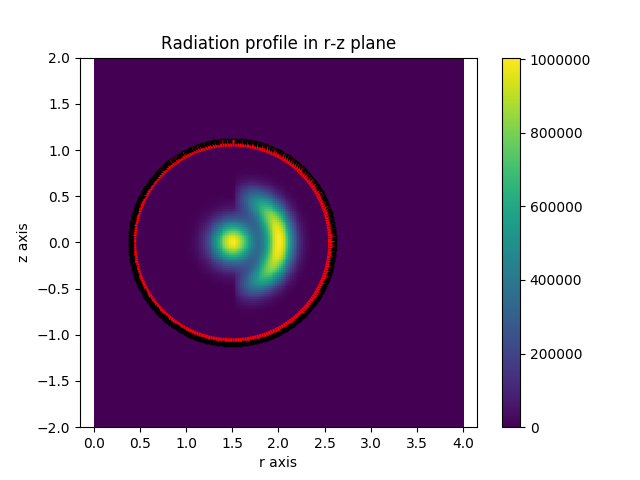
Caption: The emission source function with the wall detector positions overlaid.

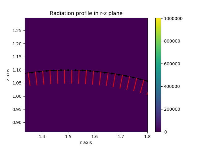
Caption: A zoomed in view of the wall detectors (black) and their surface normals (red).

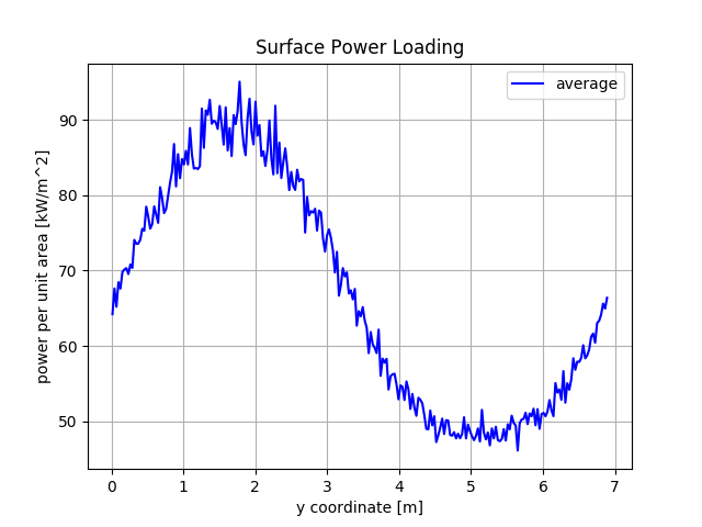
Caption: The power loading in MW/m^2 measured on the pixel detectors wrapping around the wall.