Observing a 3D Radiation Function with a Bolometer
In this demonstration we forward model the measured power on a synthetic bolometer diagnostic viewing a 3D — but axisymmetric — emissivity profile. The emissivity profile is defined in the R-Z plane and then mapped to 3D world space. The bolometer system is produced in the same way as in the Camera From Primitives demo. The emitter is produced in the same way as in the Defining A Radiation Function demo, except that the emission profile is a torus with circular cross section and uniform emissivity of 1W/m³.
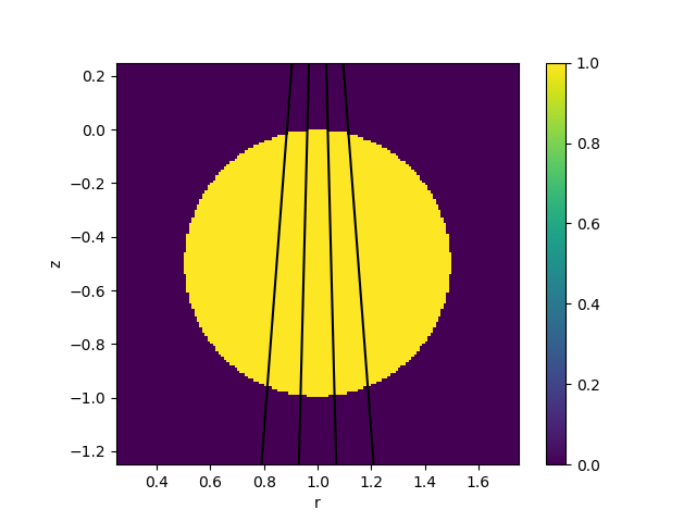
Caption A slice through the 3D emission function in the R-Z plane, along with the lines of sight of the bolometer foils.
5 measurements are presented:
Power measured on the foil
Radiance measured by a single line of sight observer
Radiance measured on the foil, using the volumetric power divided by the etendue
Radiance measured on the foil, using the radiance pipeline
Brightness measured on the foil, assuming the power is radiated isotropically
Note that the radiance pipeline measures the radiance averaged over the entire solid angle of the detector, which is \(2\pi\) steradians for a bolometer foil. To get a meaningful comparison with the sightline observer we need to renormalise to the fractional solid angle subtended by the foil-slit system. This is described in more detail in the Bolometry section of the documentation.
"""
This example demonstrates creating a radiating object with radiation
defined as a 3D function f(x, y, z), and observing that radiation with
the bolometers. Note that in this case the 3D radiation profile is
produced by defining an axisymmetric 2D profile and mapping that to 3D.

5 measurements are presented:
- Power measured on the foil
- Radiance measured by a single line of sight observer
- Radiance measured on the foil, using the volumetric power divided by
  the etendue
- Radiance measured on the foil, using the radiance pipeline
- Brightness measured on the foil, assuming the power is radiated
  isotropically

Note that the radiance pipeline measures the radiance averaged over the
entire solid angle of the detector, which is 2pi steradians for a
bolometer foil. To get a meaningful comparison with the sightline
observer we need to renormalise to the fractional solid angle subtended
by the foil-slit system.
"""
import math
import matplotlib.pyplot as plt

from raysect.core import Node, Point2D, Point3D, Vector3D, rotate_basis, translate
from raysect.optical import World
from raysect.optical.material import AbsorbingSurface, VolumeTransform
from raysect.primitive import Box, Cylinder, Subtract

from cherab.core.math import AxisymmetricMapper, sample2d
from cherab.tools.emitters import RadiationFunction
from cherab.tools.observers.bolometry import BolometerCamera, BolometerSlit, BolometerFoil


# Convenient constants
XAXIS = Vector3D(1, 0, 0)
YAXIS = Vector3D(0, 1, 0)
ZAXIS = Vector3D(0, 0, 1)
ORIGIN = Point3D(0, 0, 0)
# Bolometer geometry
BOX_WIDTH = 0.05
BOX_HEIGHT = 0.07
BOX_DEPTH = 0.2
SLIT_WIDTH = 0.004
SLIT_HEIGHT = 0.005
FOIL_WIDTH = 0.0013
FOIL_HEIGHT = 0.0038
FOIL_CORNER_CURVATURE = 0.0005
SLIT_SENSOR_SEPARATION = 0.1
FOIL_SEPARATION = 0.00508  # 0.2 inch between foils

world = World()

########################################################################
# Build a simple bolometer camera.
########################################################################

# The camera consists of a box with a rectangular slit and 4 foils.
# In its local coordinate system, the camera's slit is located at the
# origin and the foils below the z=0 plane, looking up towards the slit.
camera_box = Box(lower=Point3D(-BOX_WIDTH / 2, -BOX_HEIGHT / 2, -BOX_DEPTH),
                 upper=Point3D(BOX_WIDTH / 2, BOX_HEIGHT / 2, 0))
# Hollow out the box
inside_box = Box(lower=camera_box.lower + Vector3D(1e-5, 1e-5, 1e-5),
                 upper=camera_box.upper - Vector3D(1e-5, 1e-5, 1e-5))
camera_box = Subtract(camera_box, inside_box)
# The slit is a hole in the box
aperture = Box(lower=Point3D(-SLIT_WIDTH / 2, -SLIT_HEIGHT / 2, -1e-4),
               upper=Point3D(SLIT_WIDTH / 2, SLIT_HEIGHT / 2, 1e-4))
camera_box = Subtract(camera_box, aperture)
camera_box.material = AbsorbingSurface()
# Instance of the bolometer camera
bolometer_camera = BolometerCamera(camera_geometry=camera_box)
# The bolometer slit in this instance just contains targeting information
# for the ray tracing, since we have already given our camera a geometry
# The slit is defined in the local coordinate system of the camera
slit = BolometerSlit(slit_id="Example slit", centre_point=ORIGIN,
                     basis_x=XAXIS, dx=SLIT_WIDTH, basis_y=YAXIS, dy=SLIT_HEIGHT,
                     parent=bolometer_camera, csg_aperture=False)
# 4 bolometer foils, spaced at equal intervals along the local X axis
# The bolometer positions and orientations are given in the local coordinate
# system of the camera, just like the slit
sensor = Node(name="Bolometer sensor", parent=bolometer_camera,
              transform=translate(0, 0, -SLIT_SENSOR_SEPARATION))
# The foils are shifted relative to the centre of the sensor by -1.5, -0.5, 0.5 and 1.5
# times the foil-foil separation
for i, shift in enumerate([-1.5, -0.5, 0.5, 1.5]):
    foil_transform = translate(shift * FOIL_SEPARATION, 0, 0) * sensor.transform
    foil = BolometerFoil(detector_id="Foil {}".format(i + 1),
                         centre_point=ORIGIN.transform(foil_transform),
                         basis_x=XAXIS.transform(foil_transform), dx=FOIL_WIDTH,
                         basis_y=YAXIS.transform(foil_transform), dy=FOIL_HEIGHT,
                         slit=slit, parent=bolometer_camera, units="Power",
                         accumulate=False, curvature_radius=FOIL_CORNER_CURVATURE)
    bolometer_camera.add_foil_detector(foil)

bolometer_camera.transform = translate(1, 0, 1.5) * rotate_basis(-ZAXIS, YAXIS)
bolometer_camera.parent = world

########################################################################
# Produce a simple radiating plasma.
########################################################################

# The plasma will be a cylindrical plasma which emits with a constant
# emissivity of 1 W/m3 in an annular ring.
# See the RadiationFunction example for more details of how this is set up.
MAJOR_RADIUS = 1
MINOR_RADIUS = 0.5
CENTRE_Z = -0.5
CYLINDER_HEIGHT = 5
EMISSIVITY = 1

def emission_function(r, z):
    if (r - MAJOR_RADIUS)**2 + (z - CENTRE_Z)**2 < MINOR_RADIUS**2:
        return EMISSIVITY
    return 0

emitter = Cylinder(radius=MAJOR_RADIUS + MINOR_RADIUS, height=CYLINDER_HEIGHT,
                   transform=translate(0, 0, CENTRE_Z - CYLINDER_HEIGHT / 2))
emission_function_3d = AxisymmetricMapper(emission_function)
emitting_material = VolumeTransform(RadiationFunction(emission_function_3d),
                                    transform=emitter.transform.inverse())
emitter.material = emitting_material

########################################################################
# Plot the bolometer lines of sight and the radiation function
########################################################################
floor = Box(lower=Point3D(-10, -10, -1.26), upper=Point3D(10, 10, -1.25), parent=world,
            material=AbsorbingSurface(), name="Z=-1.25 plane")


def _point3d_to_rz(point):
    return Point2D(math.hypot(point.x, point.y), point.z)


fig, ax = plt.subplots()
for foil in bolometer_camera:
    slit_centre = foil.slit.centre_point
    slit_centre_rz = _point3d_to_rz(slit_centre)
    ax.plot(slit_centre_rz[0], slit_centre_rz[1], 'ko')
    origin, hit, _ = foil.trace_sightline()
    centre_rz = _point3d_to_rz(foil.centre_point)
    ax.plot(centre_rz[0], centre_rz[1], 'kx')
    origin_rz = _point3d_to_rz(origin)
    hit_rz = _point3d_to_rz(hit)
    ax.plot([origin_rz[0], hit_rz[0]], [origin_rz[1], hit_rz[1]], 'k')

r, z, emiss_sampled = sample2d(
    emission_function, (0.25, 1.75, 150), (-1.25, 0.25, 150)
)
image = ax.imshow(emiss_sampled.T, origin="lower", zorder=-10,
                  extent=(r.min(), r.max(), z.min(), z.max()))
fig.colorbar(image)
ax.set_xlabel("r")
ax.set_ylabel("z")


########################################################################
# Measure the radiation with the bolometers
########################################################################

emitter.parent = world

for foil in bolometer_camera:
    # Ensure reasonable sampling statistics
    foil.pixel_samples = 100000
    # Measure the incident power
    foil.units = "Power"
    foil.observe()
    power = foil.pipelines[0].value.mean
    power_error = foil.pipelines[0].value.error()
    print("Measured power for {}:\t\t{:.03g} +- {:.1g} W".format(foil.name, power, power_error))
    # Measure the incident radiance with a sightline
    foil.units = "Radiance"
    sightline = foil.as_sightline()
    sightline.observe()
    sightline_radiance = sightline.pipelines[0].value.mean
    print("Sightline radiance for {}:\t\t{:.03g} W/m2/sr".format(sightline.name, sightline_radiance))
    # Calculate the incident radiance from the power
    emitter.parent = None  # No other objects should be in the scene for etendue calculation
    floor.parent = None
    etendue, etendue_error = foil.calculate_etendue()
    radiance_from_power = power / etendue
    radiance_from_power_error = (math.hypot(power_error / power, etendue_error / etendue)
                                 * radiance_from_power)
    print("Radiance from power for {}:\t\t{:.03g} +- {:.1g} W/m2/sr".format(
        foil.name, radiance_from_power, radiance_from_power_error))
    # Calculate the incident radiance directly, renormalising for comparison with the sightline
    emitter.parent = world
    foil.units = "Radiance"
    foil.observe()
    fractional_solid_angle = etendue / foil.sensitivity
    radiance = foil.pipelines[0].value.mean / fractional_solid_angle
    radiance_error = (
        math.hypot(foil.pipelines[0].value.error() / foil.pipelines[0].value.mean,
                   etendue_error / etendue)
        * radiance
    )
    print("Measured radiance for {}:\t\t{:.03g} +- {:.1g} W/m2/sr".format(
        foil.name, radiance, radiance_error))
    # Calculate the brightness, assuming power is radiated isotropically in 4pi steradians
    brightness = radiance * 4 * math.pi
    brightness_error = radiance_error / radiance * brightness
    print("Calculated brightness for {}:\t{:.03g} +- {:.1g} W/m2".format(
        foil.name, brightness, brightness_error))
    print()

plt.show()
The demo prints the following output (note that subsequent runs may have slightly different numbers due to random sampling of the emitting material):
Measured power for Foil 1:          7.55e-10 +- 2e-12 W
Sightline radiance for Foil 1:      0.0813 W/m2/sr
Radiance from power for Foil 1:     0.081 +- 0.0007 W/m2/sr
Measured radiance for Foil 1:       0.0721 +- 0.0006 W/m2/sr
Calculated brightness for Foil 1:   0.906 +- 0.008 W/m2

Measured power for Foil 2:          6.93e-10 +- 2e-12 W
Sightline radiance for Foil 2:      0.0716 W/m2/sr
Radiance from power for Foil 2:     0.0735 +- 0.0004 W/m2/sr
Measured radiance for Foil 2:       0.0735 +- 0.0004 W/m2/sr
Calculated brightness for Foil 2:   0.923 +- 0.005 W/m2

Measured power for Foil 3:          6.93e-10 +- 2e-12 W
Sightline radiance for Foil 3:      0.0716 W/m2/sr
Radiance from power for Foil 3:     0.0735 +- 0.0005 W/m2/sr
Measured radiance for Foil 3:       0.0736 +- 0.0005 W/m2/sr
Calculated brightness for Foil 3:   0.925 +- 0.007 W/m2

Measured power for Foil 4:          6.71e-10 +- 2e-12 W
Sightline radiance for Foil 4:      0.0718 W/m2/sr
Radiance from power for Foil 4:     0.0717 +- 0.0006 W/m2/sr
Measured radiance for Foil 4:       0.072 +- 0.0006 W/m2/sr
Calculated brightness for Foil 4:   0.905 +- 0.007 W/m2
The brightness (i.e. the integral of the emissivity along the field of view of each bolometer assuming the emission is radiated isotropically into \(4\pi\) steradians) is approximately 1W/m². The emissivity profile is a constant 1W/m³ and the emitter has a diameter of 1m, so these numbers are reasonable.