Rectangular regular grid
This example shows how to:
calculate ray transfer matrix (geometry matrix) for a rectangular emitter defined on a regular grid,
obtain images using calculated ray transfer matrix by collapsing it with various emission profiles.
Notice that RoughNickel material is imported from cherab.tools.raytransfer and not from raysect.optical.library.
# Copyright 2016-2018 Euratom
# Copyright 2016-2018 United Kingdom Atomic Energy Authority
# Copyright 2016-2018 Centro de Investigaciones Energéticas, Medioambientales y Tecnológicas
#
# Licensed under the EUPL, Version 1.1 or – as soon they will be approved by the
# European Commission - subsequent versions of the EUPL (the "Licence");
# You may not use this work except in compliance with the Licence.
# You may obtain a copy of the Licence at:
#
# https://joinup.ec.europa.eu/software/page/eupl5
#
# Unless required by applicable law or agreed to in writing, software distributed
# under the Licence is distributed on an "AS IS" basis, WITHOUT WARRANTIES OR
# CONDITIONS OF ANY KIND, either express or implied.
#
# See the Licence for the specific language governing permissions and limitations
# under the Licence.

"""
RayTransferBox Demonstration
----------------------------

This file will demonstrate how to:

 * calculate ray transfer matrix (geometry matrix) for a rectangular emitter defined
   on a regular grid,
 * obtain images by collapsing calculated ray transfer matrix with various emission profiles.

"""
import os
import numpy as np
from matplotlib import pyplot as plt

from raysect.primitive import Box
from raysect.optical import World, translate, rotate, Point3D
from raysect.optical.observer import PinholeCamera, FullFrameSampler2D

# RayTransferPipeline2D is optimised for calculation of ray transfer matrices.
# It's also possible to use SpectralRadiancePipeline2D or SpectralPowerPipeline2D but
# for the matrices with >1000 elements the performance will be lower.
from cherab.tools.raytransfer import RayTransferPipeline2D, RayTransferBox

# Here we use special materials optimised for calculation of ray transfer matrices.
# The materials from raysect.optical.library can be used as well but like in the case of pipeline
# the performance will be lower for large ray transfer matrices.
from cherab.tools.raytransfer import RoughNickel

world = World()

# creating the scene
ground = Box(lower=Point3D(-150, -14.2, -100), upper=Point3D(150, -14.1, 150),
             material=RoughNickel(0.1), parent=world)
wall = Box(lower=Point3D(-150, -150, 44.1), upper=Point3D(150, 150, 44.2),
           material=RoughNickel(0.1), parent=world)

# creating ray transfer box with size of 120 (m) x 80 (m) x 10 (m) for emission profile
# defined on a 12 x 8 x 1 gird
rtb = RayTransferBox(120., 80., 10., 12, 8, 1, transform=translate(-60., 0, 0), parent=world)
# like any primitive, the box can be connected to scenegraph or transformed at any moment,
# not only at initialisation

# rtb.parent = world
# rtb.transform = translate(-60., 0, 0)

# setting the integration step (can be done at initialisation)
rtb.step = 0.2

# creating ray transfer pipeline
# Be careful when setting the 'kind' attribute of the pipeline to 'power' or 'radiance'.
# In the case of 'power', the matrix [m] is multiplied by the detector's sensitivity [m^2 sr].
# For the PinholeCamera this does not matter, because its pixel sensitivity is 1.
pipeline = RayTransferPipeline2D()

# setting up the camera
camera = PinholeCamera((256, 256), pipelines=[pipeline], frame_sampler=FullFrameSampler2D(),
                       transform=rotate(-15., -35, 0) * translate(-10, 50, -250), parent=world)
camera.fov = 45
camera.pixel_samples = 1000
camera.min_wavelength = 500.
camera.max_wavelength = camera.min_wavelength + 1.
# Ray transfer matrices are calculated for a single value of wavelength,
# but the number of spectral bins must be equal to the number of active voxels in the grid.
# This is so because the spectral array is used to store the values of ray transfer matrix.
camera.spectral_bins = rtb.bins

# starting ray tracing
camera.observe()

# let's collapse the ray transfer matrix with some emission profiles

# defining emission profiles on a 12 x 8 x 1 grid
profiles = [np.array([[[0, 0, 1, 1, 0, 0, 0, 1, 1, 0, 0, 0],
                       [1, 0, 1, 0, 0, 0, 0, 0, 1, 0, 1, 0],
                       [1, 0, 1, 1, 1, 1, 1, 1, 1, 0, 1, 0],
                       [1, 1, 1, 1, 1, 1, 1, 1, 1, 1, 1, 0],
                       [0, 1, 1, 0, 1, 1, 1, 0, 1, 1, 0, 0],
                       [0, 0, 1, 1, 1, 1, 1, 1, 1, 0, 0, 0],
                       [0, 0, 0, 1, 0, 0, 0, 1, 0, 0, 0, 0],
                       [0, 0, 1, 0, 0, 0, 0, 0, 1, 0, 0, 0]]], dtype=np.float64).T,

            np.array([[[0, 1, 0, 0, 0, 0, 0, 0, 0, 1, 0, 0],
                       [0, 0, 1, 0, 0, 0, 0, 0, 1, 0, 0, 0],
                       [0, 1, 1, 1, 1, 1, 1, 1, 1, 1, 0, 0],
                       [1, 1, 1, 1, 1, 1, 1, 1, 1, 1, 1, 0],
                       [1, 1, 1, 0, 1, 1, 1, 0, 1, 1, 1, 0],
                       [1, 0, 1, 1, 1, 1, 1, 1, 1, 0, 1, 0],
                       [1, 0, 0, 1, 0, 0, 0, 1, 0, 0, 1, 0],
                       [0, 0, 1, 0, 0, 0, 0, 0, 1, 0, 0, 0]]], dtype=np.float64).T,

            np.array([[[0, 0, 1, 0, 1, 0, 0, 1, 0, 1, 0, 0],
                       [0, 0, 0, 1, 0, 1, 1, 0, 1, 0, 0, 0],
                       [0, 0, 0, 0, 1, 0, 0, 1, 0, 0, 0, 0],
                       [0, 0, 1, 1, 1, 1, 1, 1, 1, 1, 0, 0],
                       [0, 0, 1, 1, 0, 1, 1, 0, 1, 1, 0, 0],
                       [0, 0, 0, 1, 1, 1, 1, 1, 1, 0, 0, 0],
                       [0, 0, 0, 0, 1, 1, 1, 1, 0, 0, 0, 0],
                       [0, 0, 0, 0, 0, 1, 1, 0, 0, 0, 0, 0]]], dtype=np.float64).T,

            np.array([[[0, 0, 1, 1, 0, 0, 0, 0, 1, 1, 0, 0],
                       [0, 1, 1, 0, 0, 1, 1, 0, 0, 1, 1, 0],
                       [0, 0, 1, 1, 1, 0, 0, 1, 1, 1, 0, 0],
                       [1, 1, 1, 1, 1, 1, 1, 1, 1, 1, 1, 1],
                       [1, 1, 1, 0, 0, 1, 1, 0, 0, 1, 1, 1],
                       [1, 1, 1, 1, 1, 1, 1, 1, 1, 1, 1, 1],
                       [0, 1, 1, 1, 1, 1, 1, 1, 1, 1, 1, 0],
                       [0, 0, 0, 0, 1, 1, 1, 1, 0, 0, 0, 0]]], dtype=np.float64).T]

# obtaining the images by collapsing the ray transfer matrix with emission profiles
# note that ptofiles must be flattened first
images = [np.dot(pipeline.matrix, profile.flatten()) for profile in profiles]

# creating a folder for images
if not os.path.exists('images'):
    os.makedirs('images')

# now let's see 4 diffrent ray-traced images obtained with only a single run of ray-tracing
fig = plt.figure(figsize=(6., 6.))
for i in range(4):
    ax = fig.add_subplot(2, 2, i + 1)
    ax.imshow(images[i].T, cmap='gray')
    ax.tick_params(labelbottom=False, labelleft=False, bottom=False, left=False)
fig.subplots_adjust(left=0.05, right=0.95, bottom=0.05, top=0.95, wspace=0.05, hspace=0.05)
fig.savefig('images/ray_transfer_box_demo.png', dpi=180)
plt.show()
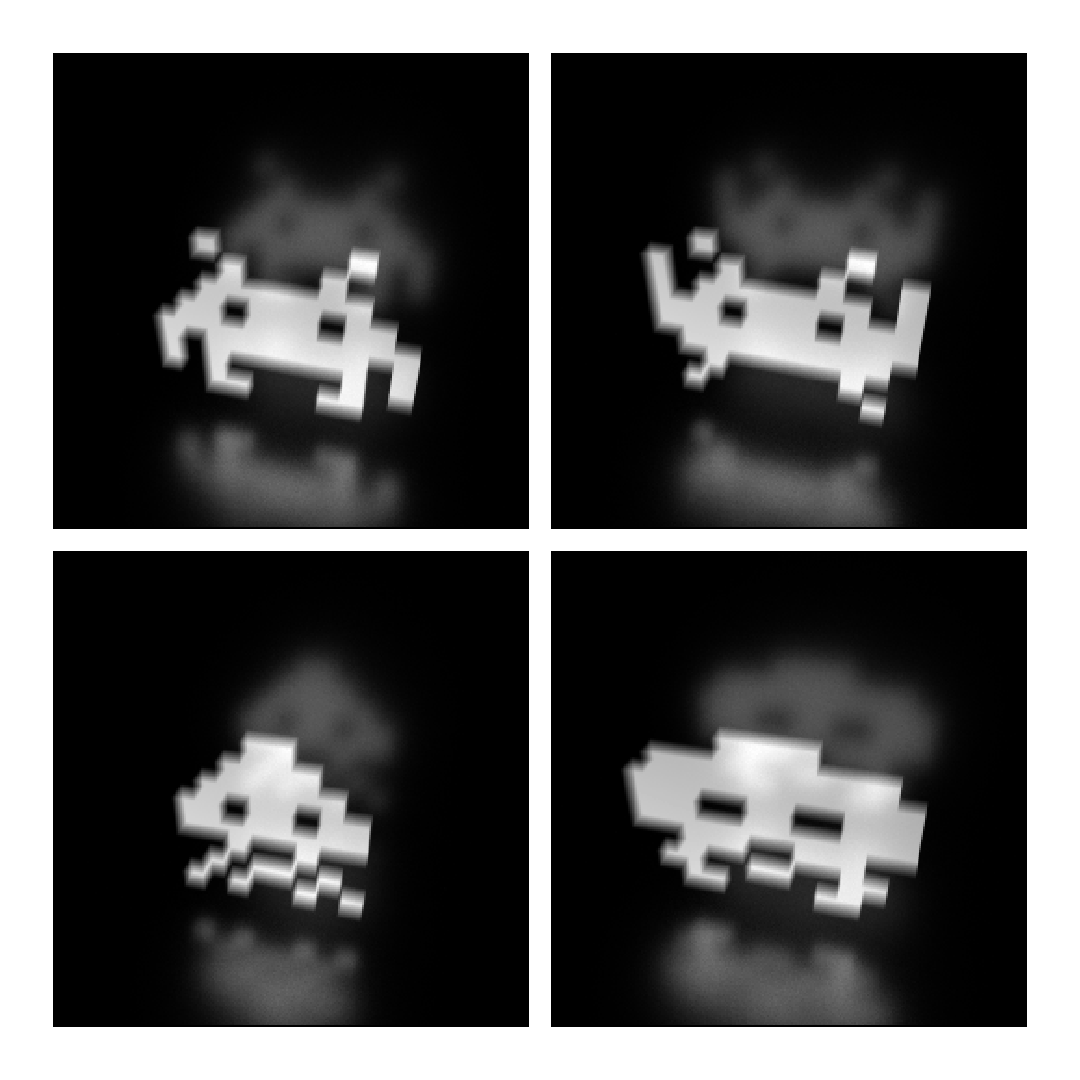
Caption: The result of collapsing geometry matrix with four different emission profiles.