2D Mesh Plasmas

This demonstration shows how to define a set of plasma distributions using 2D meshes that are revolved around the z-axis. This use case is commonly encountered when we already have a plasma solution that has been computed with a fluid code or particle-in-cell code. These codes typically export their plasma solutions on a mesh in a 2D plane, assuming a symmetry axis. The plasma values are defined either at the mesh vertices or inside the cells.

These types of plasmas can be achieved in Cherab with Raysect’s mesh interpolators, Discrete2DMesh and Interpolator2DMesh. Both mesh functions are defined on a triangular mesh. The mesh vertex coordinates and triangle definitions are given as arguments. The Discrete2DMesh defines it’s values as constant inside each triangle, with the triangle values supplied as an argument. The Interpolator2DMesh takes values defined at the triangle vertices and performs Barycentric interpolation within each triangle. Both 2D mesh functions can be promoted to 3D functions with the AxisymmetricMapper class, which maps a 2D r-z function around the z-axis.

In this example we create a simple triangular mesh from scratch and sample some analytic functions describing a cylindrically symmetric plasma column at the mesh vertices. However, in real use cases you would use the mesh description supplied by the plasma simulation code.

# Copyright 2016-2018 Euratom
# Copyright 2016-2018 United Kingdom Atomic Energy Authority
# Copyright 2016-2018 Centro de Investigaciones Energéticas, Medioambientales y Tecnológicas
#
# Licensed under the EUPL, Version 1.1 or – as soon they will be approved by the
# European Commission - subsequent versions of the EUPL (the "Licence");
# You may not use this work except in compliance with the Licence.
# You may obtain a copy of the Licence at:
#
# https://joinup.ec.europa.eu/software/page/eupl5
#
# Unless required by applicable law or agreed to in writing, software distributed
# under the Licence is distributed on an "AS IS" basis, WITHOUT WARRANTIES OR
# CONDITIONS OF ANY KIND, either express or implied.
#
# See the Licence for the specific language governing permissions and limitations
# under the Licence.


import numpy as np
import matplotlib.pyplot as plt
from scipy.constants import electron_mass, atomic_mass
from scipy.spatial import Delaunay

from raysect.core.math.function.float import Interpolator2DMesh
from raysect.primitive import Cylinder
from raysect.optical import World, translate, Point3D, Vector3D, rotate_basis, Spectrum
from raysect.optical.observer import PinholeCamera, PowerPipeline2D

from cherab.core import Species, Maxwellian, Plasma, Line
from cherab.core.math import sample3d, AxisymmetricMapper
from cherab.core.atomic import deuterium
from cherab.core.model import ExcitationLine, RecombinationLine
from cherab.openadas import OpenADAS


# tunable parameters
peak_density = 1e19
peak_temperature = 2500


def neutral_distribution(r, peak, lcfs_radius=1, sigma=0.1):
    """A neutral profile that is constant outside the plasma,
       then exponentially decays inside the LCFS."""

    if r <= lcfs_radius:
        return peak * np.exp(-((r - lcfs_radius) ** 2) / (2*sigma**2))
    else:
        return peak


def ion_distribution(r, v_core, v_lcfs, p=4, q=3, lcfs_radius=1):
    """A cylindrical plasma profile that follows a double
       quadratic between the LCFS and axisymmetric z axis."""

    # evaluate pedestal-> core function
    if r <= lcfs_radius:
        return ((v_core - v_lcfs) *
                np.power((1 - np.power(r / lcfs_radius, p)), q) + v_lcfs)
    else:
        return 0


####################
# 2D Mesh creation #

# Make a triangular mesh in the r-z plane

num_vertical_points = 100
vertical_points = np.linspace(-2, 2, num_vertical_points)
num_radial_points = 30
radial_points = np.linspace(0, 1.5, num_radial_points)

vertex_coords = np.empty((num_vertical_points * num_radial_points, 2))
for i in range(num_radial_points):
    for j in range(num_vertical_points):
        index = i * num_vertical_points + j
        vertex_coords[index, 0] = radial_points[i]
        vertex_coords[index, 1] = vertical_points[j]

# perform Delaunay triangulation to produce triangular mesh
triangles = Delaunay(vertex_coords).simplices

# sample our plasma functions at the mesh vertices
d0_vertex_densities = np.array([neutral_distribution(r, peak_density) for r, z in vertex_coords])
d1_vertex_densities = np.array([ion_distribution(r, peak_density, 0) for r, z in vertex_coords])
d1_vertex_temperatures = np.array([ion_distribution(r, peak_temperature, 0) for r, z in vertex_coords])


###################
# plasma creation #

world = World()  # setup scenegraph

plasma = Plasma(parent=world)
plasma.atomic_data = OpenADAS(permit_extrapolation=True)
plasma.geometry = Cylinder(1.5, 4, transform=translate(0, 0, -2))
plasma.geometry_transform = translate(0, 0, -2)

# No net velocity for any species
zero_velocity = Vector3D(0, 0, 0)

# define neutral species distribution

# create a 2D interpolator from the mesh coords and data samples
d0_density_interp = Interpolator2DMesh(vertex_coords, d0_vertex_densities, triangles, limit=False)
# map the 2D interpolator into a 3D function using the axisymmetry operator
d0_density = AxisymmetricMapper(d0_density_interp)
d0_temperature = 0.5  # constant 0.5eV temperature for all neutrals
d0_distribution = Maxwellian(d0_density, d0_temperature, zero_velocity,
                             deuterium.atomic_weight * atomic_mass)
d0_species = Species(deuterium, 0, d0_distribution)

# define deuterium ion species distribution
d1_density_interp = Interpolator2DMesh(vertex_coords, d1_vertex_densities, triangles, limit=False)
d1_density = AxisymmetricMapper(d1_density_interp)
d1_temperature_interp = Interpolator2DMesh(vertex_coords, d1_vertex_temperatures, triangles, limit=False)
d1_temperature = AxisymmetricMapper(d1_temperature_interp)
d1_distribution = Maxwellian(d1_density, d1_temperature, zero_velocity,
                             deuterium.atomic_weight * atomic_mass)
d1_species = Species(deuterium, 1, d1_distribution)

# define the electron distribution
e_density_interp = Interpolator2DMesh(vertex_coords, d1_vertex_densities, triangles, limit=False)
e_density = AxisymmetricMapper(e_density_interp)
e_temperature_interp = Interpolator2DMesh(vertex_coords, d1_vertex_temperatures, triangles, limit=False)
e_temperature = AxisymmetricMapper(e_temperature_interp)
e_distribution = Maxwellian(e_density, e_temperature, zero_velocity, electron_mass)

# define species
plasma.b_field = Vector3D(1.0, 1.0, 1.0)
plasma.electron_distribution = e_distribution
plasma.composition = [d0_species, d1_species]

# Add a balmer alpha line for visualisation purposes
d_alpha_excit = ExcitationLine(Line(deuterium, 0, (3, 2)))
plasma.models = [d_alpha_excit]


####################
# Visualise Plasma #

# Run some plots to check the distribution functions and emission profile are as expected
plt.figure()
r, _, z, t_samples = sample3d(d1_temperature, (0, 1.5, 200), (0, 0, 1), (-2, 2, 200))
plt.imshow(np.transpose(np.squeeze(t_samples)), extent=[0, 1.5, -2, 2])
plt.colorbar()
plt.axis('equal')
plt.xlabel('r axis')
plt.ylabel('z axis')
plt.title("Ion temperature profile in r-z plane")

plt.figure()
r, _, z, t_samples = sample3d(d1_temperature, (-2, 2, 400), (-2, 2, 400), (0, 0, 1))
plt.imshow(np.transpose(np.squeeze(t_samples)), extent=[-2, 2, -2, 2])
plt.colorbar()
plt.axis('equal')
plt.xlabel('x axis')
plt.ylabel('y axis')
plt.title("Ion temperature profile in x-y plane")

plt.figure()
r, _, z, t_samples = sample3d(d0_density, (0, 1.5, 200), (0, 0, 1), (-2, 2, 200))
plt.imshow(np.transpose(np.squeeze(t_samples)), extent=[0, 1.5, -2, 2])
plt.colorbar()
plt.axis('equal')
plt.xlabel('r axis')
plt.ylabel('z axis')
plt.title("Neutral Density profile in r-z plane")

plt.figure()
xrange = np.linspace(-2, 2, 200)
yrange = np.linspace(-2, 2, 200)
d_alpha_rz_intensity = np.zeros((200, 200))
direction = Vector3D(0, 1, 0)
for i, x in enumerate(xrange):
    for j, y in enumerate(yrange):
        emission = d_alpha_excit.emission(Point3D(x, y, 0.0), direction, Spectrum(650, 660, 1))
        d_alpha_rz_intensity[j, i] = emission.total()
plt.imshow(d_alpha_rz_intensity, extent=[-2, 2, -2, 2], origin='lower')
plt.colorbar()
plt.xlabel('x axis')
plt.ylabel('y axis')
plt.title("D-alpha emission in x-y")


camera = PinholeCamera((256, 256), pipelines=[PowerPipeline2D()], parent=world)
camera.transform = translate(-3, 0, 0)*rotate_basis(Vector3D(1, 0, 0), Vector3D(0, 0, 1))
camera.pixel_samples = 1

plt.ion()
camera.observe()
plt.ioff()
plt.show()


# this code can be used to plot the mesh, but it's quite slow
# for tri_index in range(triangles.shape[0]):
#     v1, v2, v3 = triangles[tri_index]
#     plt.plot([vertex_coords[v1, 0], vertex_coords[v2, 0], vertex_coords[v3, 0], vertex_coords[v1, 0]],
#              [vertex_coords[v1, 1], vertex_coords[v2, 1], vertex_coords[v3, 1], vertex_coords[v1, 1]], 'k')
#     plt.plot([vertex_coords[v1, 0], vertex_coords[v2, 0], vertex_coords[v3, 0], vertex_coords[v1, 0]],
#              [vertex_coords[v1, 1], vertex_coords[v2, 1], vertex_coords[v3, 1], vertex_coords[v1, 1]], '.b')

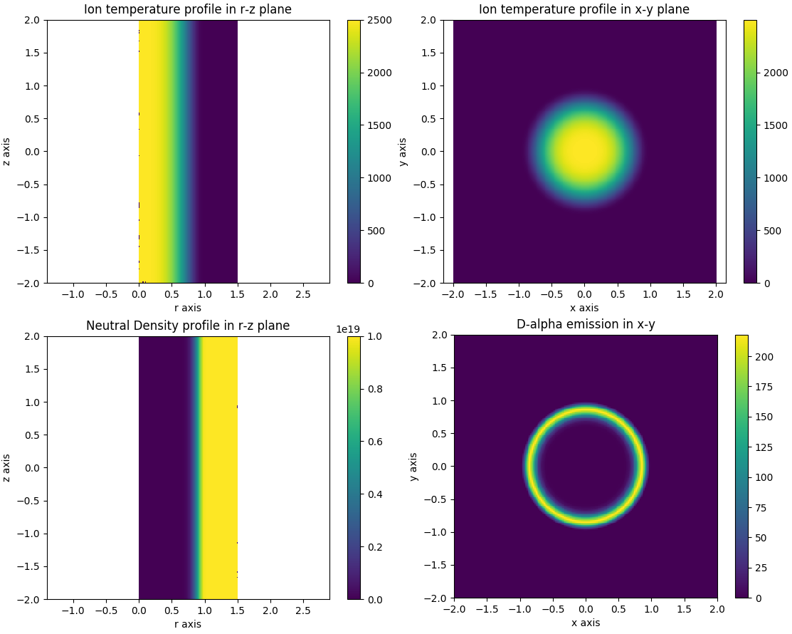
Caption: Visualisation plots of slices through the plasma.

Caption: A camera rendering of the d-alpha light from the cylindrically symmetric plasma column.

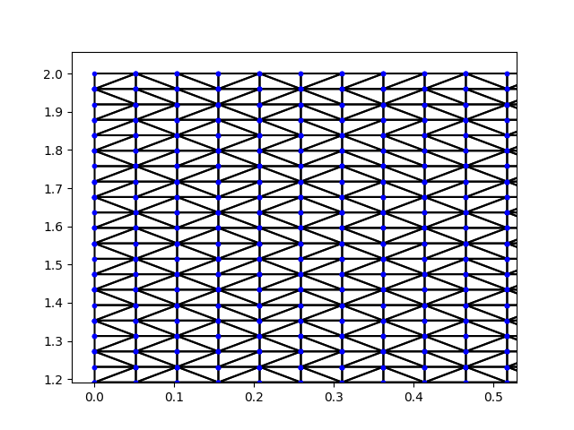
Caption: A visualisation of the underlying triangular mesh in the r-z plane. The plasma values were defined at the triangle vertices.