Flux Function Plasmas
It is a common use case to approximate the core plasma of a tokamak with 1D flux functions. For example, we might assume the electron temperature can be defined as a 1D profile function of \(\psi_n\), i.e. is constant on flux surfaces. This demonstration shows how to define plasma distributions in terms of 1D flux functions using the EFITEquilibrium’s mapping utilities.
The EFITEquilibrium class is the workhorse class
for working with tokamak equilibria in Cherab. To use equilibria in your code you
should extract the appropriate data from your equilibrium code of choice and instantiate
this class directly for a given time slice. We include an example equilibrium with the
Cherab tools module for the tutorials and experimentation.
# Copyright 2016-2018 Euratom
# Copyright 2016-2018 United Kingdom Atomic Energy Authority
# Copyright 2016-2018 Centro de Investigaciones Energéticas, Medioambientales y Tecnológicas
#
# Licensed under the EUPL, Version 1.1 or – as soon they will be approved by the
# European Commission - subsequent versions of the EUPL (the "Licence");
# You may not use this work except in compliance with the Licence.
# You may obtain a copy of the Licence at:
#
# https://joinup.ec.europa.eu/software/page/eupl5
#
# Unless required by applicable law or agreed to in writing, software distributed
# under the Licence is distributed on an "AS IS" basis, WITHOUT WARRANTIES OR
# CONDITIONS OF ANY KIND, either express or implied.
#
# See the Licence for the specific language governing permissions and limitations
# under the Licence.

"""
EFIT Equilibrium Object Demonstration
-------------------------------------

This file will demonstrate how to:

 * access equilibrium attributes
 * map functions onto flux surfaces (2d and 3d)

"""


import matplotlib.pyplot as plt
from raysect.core.math.function.float import Interpolator1DArray
from cherab.core.math import sample2d, Slice3D
from cherab.tools.equilibrium import example_equilibrium, plot_equilibrium


# populate and return an example equilibrium object.
print('Populating example equilibrium object...')
equilibrium = example_equilibrium()

# the cherab package has a convenience tool for viewing an equilibrium
# this function samples the various equilibrium attributes and renders them as images
print('Plotting equilibrium data...')
plot_equilibrium(equilibrium, detail=True)

# The core equilibrium properties are accessible as attributes on the the equilibrium object.
# For a full list of available attributes, see the object itself

# Psi and normalised psi are returned as 2D functions (see cherab.core.math.function.Function2D),
# they are cubically interpolated version of the raw gridded data. e.g. to obtain a value of psi
# normalised at the point (r=2.1m, z=0.2m), simply call the function:
psi_n = equilibrium.psi_normalised(2.1, 0.2)
print('Psi normalised at (2.1, 0.2)m: {}'.format(psi_n))

# The magnetic field is similarly accessible, it is returned as a 2D vector function. e.g. to
# obtain the components of the field at the point (r=2.1m, z=0.2m), simply call the function:
b = equilibrium.b_field(2.1, 0.2)
print('B-field at (2.1, 0.2)m: {}'.format(b))

# The inside_lcfs attribute returns a 2D function that identifies if a point lies inside the
# last closed flux surface. The function returns a value of 1.0 inside and a value of 0.0
# outside the LCFS.
print('Inside LCFS at (2.1, 0.2)m: {}'.format(equilibrium.inside_lcfs(2.1, 0.2)))
print('Inside LCFS at (2.1, 1.5)m: {}'.format(equilibrium.inside_lcfs(2.1, 1.5)))

# The equilibrium object includes methods for mapping functions onto the flux surfaces.
# These create 2D or 3D functions or e.g. temperature, density etc... according to the profile
# being mapped. The user can supply either a python function (with 1 argument - normalised psi),
# a Function1D object or a numerical array holding the normalised psi and function values.

# In this example we create fake 2D and 3D "temperature" profiles from an array of data. The
# array is interpolated with cubic interpolation and then mapped onto the normalised psi grid.
temperature_2d = equilibrium.map2d([[0, 0.5, 0.9, 1.0], [2500, 2000, 1000, 0]])
temperature_3d = equilibrium.map3d([[0, 0.5, 0.9, 1.0], [2500, 2000, 1000, 0]])

# display 2D temperature
print("Plotting array based 2d temperature...")

rmin, rmax = equilibrium.r_range
zmin, zmax = equilibrium.z_range
nr = round((rmax - rmin) / 0.025)
nz = round((zmax - zmin) / 0.025)
r, z, temperature_grid = sample2d(temperature_2d, (rmin, rmax, nr), (zmin, zmax, nz))

plt.figure()
plt.axes(aspect='equal')
plt.pcolormesh(r, z, temperature_grid.transpose(), shading='gouraud')
plt.autoscale(tight=True)
plt.colorbar()
plt.title('2D Temperature (array)')

# display 3D temperature
print("Plotting array based 3d temperature...")

rmin, rmax = equilibrium.r_range
zmin, zmax = equilibrium.z_range
nr = round((rmax - rmin) / 0.025)
nz = round((zmax - zmin) / 0.025)
temperature_slice = Slice3D(temperature_3d, axis='z', value=0.0)
x, y, temperature_grid = sample2d(temperature_slice, (-rmax, rmax, nr), (-rmax, rmax, nr))

plt.figure()
plt.axes(aspect='equal')
plt.pcolormesh(x, y, temperature_grid.transpose(), shading='gouraud')
plt.autoscale(tight=True)
plt.colorbar()
plt.title('3D Temperature (x-y slice, array)')

# In this example we interpolate the temperature data manually to produce a continuous function
# and then map that function around the flux surfaces to give the same result
te_psin = Interpolator1DArray([0, 0.5, 0.9, 1.0], [2500, 2000, 1000, 0], 'cubic', 'none', 0)

# map to produce 2D and 3D temperature profiles
temperature_2d = equilibrium.map2d(te_psin)
temperature_3d = equilibrium.map3d(te_psin)

# display 2D temperature
print("Plotting function based 2d temperature...")

rmin, rmax = equilibrium.r_range
zmin, zmax = equilibrium.z_range
nr = round((rmax - rmin) / 0.025)
nz = round((zmax - zmin) / 0.025)
r, z, temperature_grid = sample2d(temperature_2d, (rmin, rmax, nr), (zmin, zmax, nz))

plt.figure()
plt.axes(aspect='equal')
plt.pcolormesh(r, z, temperature_grid.transpose(), shading='gouraud')
plt.autoscale(tight=True)
plt.colorbar()
plt.title('2D Temperature (function)')

# display 3D temperature
print("Plotting function based 3d temperature...")

rmin, rmax = equilibrium.r_range
zmin, zmax = equilibrium.z_range
nr = round((rmax - rmin) / 0.01)
nz = round((zmax - zmin) / 0.01)
temperature_slice = Slice3D(temperature_3d, axis='z', value=0.0)
x, y, temperature_grid = sample2d(temperature_slice, (-rmax, rmax, nr), (-rmax, rmax, nr))

plt.figure()
plt.axes(aspect='equal')
plt.pcolormesh(x, y, temperature_grid.transpose(), shading='gouraud')
plt.autoscale(tight=True)
plt.colorbar()
plt.title('3D Temperature (x-y slice, function)')

plt.show()
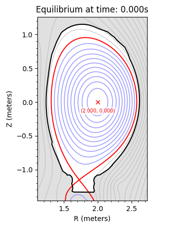
Caption: The flux surfaces of the example equilibrium.
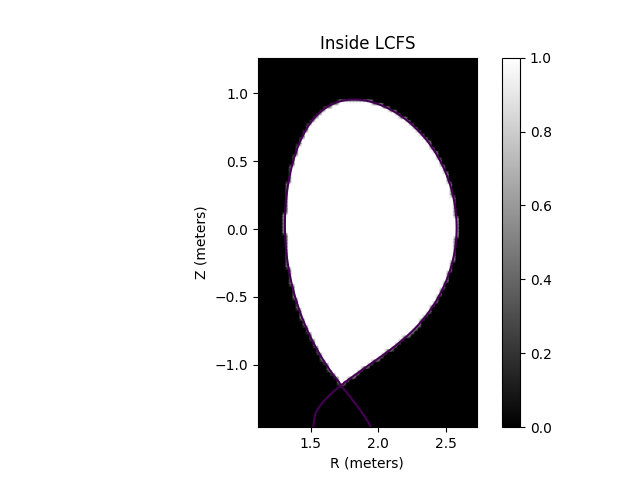
Caption: The Last Closed Flux Surface (LCFS) polygon mask.
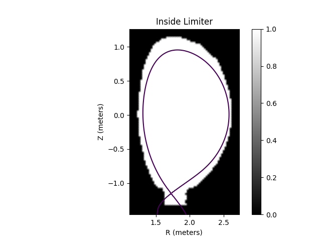
Caption: The limiter polygon mask.
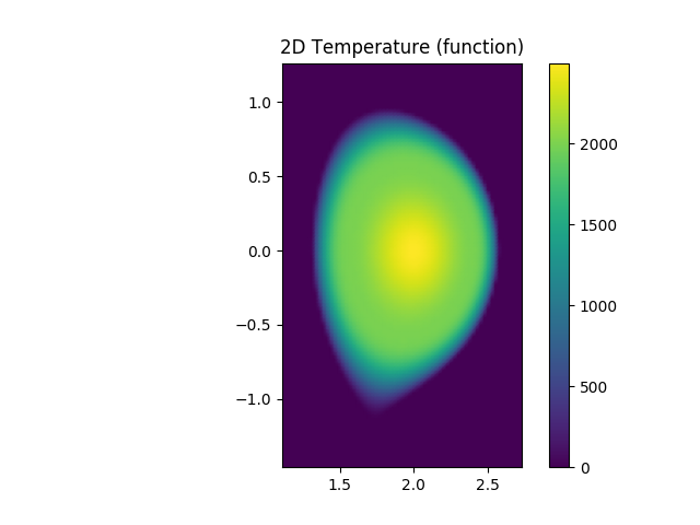
Caption: A slice of the electron temperature through the x-z plane revealing Te as a flux quantitiy.
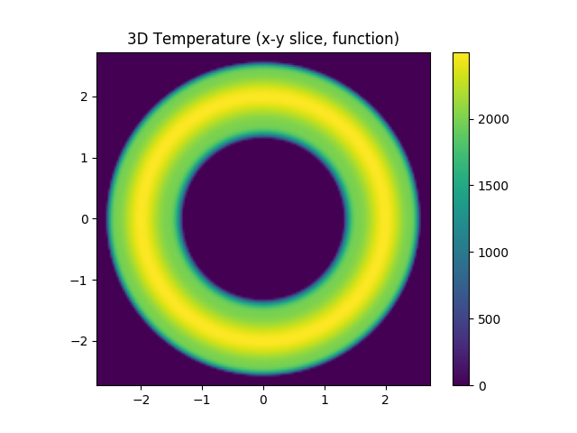
Caption: A slice of the electron temperature through the x-y plane.