Analytic Function Plasma
This demonstration shows how to define a set of plasma distributions using analytic functions. Each function must by implemented as a python callable. The rest of the code shows how to use these functions in a plasma and visualises the results.
Note that while it is possible to use pure python functions for development, they are typically ~100 times slower than their cython counterparts. Therefore, for use cases where speed is important we recommend moving these functions to cython classes. An alternative solution which may not require writing and compiling any additional cython code is to use Raysect’s function framework to build up expressions which will be evaluated like Python functions. These will typically run slightly slower than a hand-coded cython implementation but still significantly faster than a pure python implementation.
Two examples are provided, one using a pure python implementation of analytic forms for neutral and ion plasma species distributions, and one using objects from Raysect’s function framework.
# Copyright 2016-2018 Euratom
# Copyright 2016-2018 United Kingdom Atomic Energy Authority
# Copyright 2016-2018 Centro de Investigaciones Energéticas, Medioambientales y Tecnológicas
#
# Licensed under the EUPL, Version 1.1 or – as soon they will be approved by the
# European Commission - subsequent versions of the EUPL (the "Licence");
# You may not use this work except in compliance with the Licence.
# You may obtain a copy of the Licence at:
#
# https://joinup.ec.europa.eu/software/page/eupl5
#
# Unless required by applicable law or agreed to in writing, software distributed
# under the Licence is distributed on an "AS IS" basis, WITHOUT WARRANTIES OR
# CONDITIONS OF ANY KIND, either express or implied.
#
# See the Licence for the specific language governing permissions and limitations
# under the Licence.
import numpy as np
import matplotlib.pyplot as plt
from scipy.constants import electron_mass, atomic_mass
from raysect.primitive import Cylinder
from raysect.optical import World, translate, Point3D, Vector3D, rotate_basis, Spectrum
from raysect.optical.observer import PinholeCamera, PowerPipeline2D
from cherab.core import Species, Maxwellian, Plasma, Line
from cherab.core.math import sample3d
from cherab.core.atomic import deuterium
from cherab.core.model import ExcitationLine, RecombinationLine
from cherab.openadas import OpenADAS
class NeutralFunction:
"""A neutral profile that is constant outside the plasma,
then exponentially decays inside the LCFS."""
def __init__(self, peak_value, sigma, magnetic_axis, lcfs_radius=1):
self.peak = peak_value
self.sigma = sigma
self.lcfs_radius = lcfs_radius
self._constant = (2*self.sigma*self.sigma)
self.r_axis = magnetic_axis[0]
self.z_axis = magnetic_axis[1]
def __call__(self, x, y, z):
# calculate r in r-z space
r = np.sqrt(x**2 + y**2)
# calculate radius of coordinate from magnetic axis
radius_from_axis = np.sqrt((r - self.r_axis)**2 + (z - self.z_axis)**2)
if radius_from_axis <= self.lcfs_radius:
return self.peak * np.exp(-((radius_from_axis - self.lcfs_radius)**2) / self._constant)
else:
return self.peak
class IonFunction:
"""An approximate toroidal plasma profile that follows a double
quadratic between the LCFS and magnetic axis."""
def __init__(self, v_core, v_lcfs, magnetic_axis, p=4, q=3, lcfs_radius=1):
self.v_core = v_core
self.v_lcfs = v_lcfs
self.p = p
self.q = q
self.lcfs_radius = lcfs_radius
self.r_axis = magnetic_axis[0]
self.z_axis = magnetic_axis[1]
def __call__(self, x, y, z):
# calculate r in r-z space
r = np.sqrt(x**2 + y**2)
# calculate radius of coordinate from magnetic axis
radius_from_axis = np.sqrt((r - self.r_axis)**2 + (z - self.z_axis)**2)
# evaluate pedestal-> core function
if radius_from_axis <= self.lcfs_radius:
return ((self.v_core - self.v_lcfs) *
np.power((1 - np.power(radius_from_axis / self.lcfs_radius, self.p)), self.q) + self.v_lcfs)
else:
return 0
# tunables
peak_density = 1e19
peak_temperature = 2500
magnetic_axis = (2.5, 0)
# setup scenegraph
world = World()
###################
# plasma creation #
plasma = Plasma(parent=world)
plasma.atomic_data = OpenADAS(permit_extrapolation=True)
plasma.geometry = Cylinder(3.5, 2.2, transform=translate(0, 0, -1.1))
plasma.geometry_transform = translate(0, 0, -1.1)
# No net velocity for any species
zero_velocity = Vector3D(0, 0, 0)
# define neutral species distribution
d0_density = NeutralFunction(peak_density, 0.1, magnetic_axis)
d0_temperature = 0.5 # constant 0.5eV temperature for all neutrals
d0_distribution = Maxwellian(d0_density, d0_temperature, zero_velocity,
deuterium.atomic_weight * atomic_mass)
d0_species = Species(deuterium, 0, d0_distribution)
# define deuterium ion species distribution
d1_density = IonFunction(peak_density, 0, magnetic_axis)
d1_temperature = IonFunction(peak_temperature, 0, magnetic_axis)
d1_distribution = Maxwellian(d1_density, d1_temperature, zero_velocity,
deuterium.atomic_weight * atomic_mass)
d1_species = Species(deuterium, 1, d1_distribution)
# define the electron distribution
e_density = IonFunction(peak_density, 0, magnetic_axis)
e_temperature = IonFunction(peak_temperature, 0, magnetic_axis)
e_distribution = Maxwellian(e_density, e_temperature, zero_velocity, electron_mass)
# define species
plasma.b_field = Vector3D(1.0, 1.0, 1.0)
plasma.electron_distribution = e_distribution
plasma.composition = [d0_species, d1_species]
# Add a balmer alpha line for visualisation purposes
d_alpha_excit = ExcitationLine(Line(deuterium, 0, (3, 2)))
plasma.models = [d_alpha_excit]
####################
# Visualise Plasma #
# Run some plots to check the distribution functions and emission profile are as expected
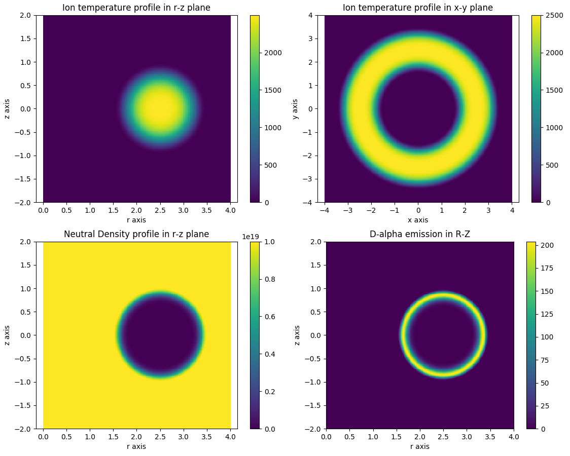
r, _, z, t_samples = sample3d(d1_temperature, (0, 4, 200), (0, 0, 1), (-2, 2, 200))
plt.imshow(np.transpose(np.squeeze(t_samples)), extent=[0, 4, -2, 2])
plt.colorbar()
plt.axis('equal')
plt.xlabel('r axis')
plt.ylabel('z axis')
plt.title("Ion temperature profile in r-z plane")
plt.figure()
r, _, z, t_samples = sample3d(d1_temperature, (-4, 4, 400), (-4, 4, 400), (0, 0, 1))
plt.imshow(np.transpose(np.squeeze(t_samples)), extent=[-4, 4, -4, 4])
plt.colorbar()
plt.axis('equal')
plt.xlabel('x axis')
plt.ylabel('y axis')
plt.title("Ion temperature profile in x-y plane")
plt.figure()
r, _, z, t_samples = sample3d(d0_density, (0, 4, 200), (0, 0, 1), (-2, 2, 200))
plt.imshow(np.transpose(np.squeeze(t_samples)), extent=[0, 4, -2, 2])
plt.colorbar()
plt.axis('equal')
plt.xlabel('r axis')
plt.ylabel('z axis')
plt.title("Neutral Density profile in r-z plane")
plt.figure()
xrange = np.linspace(0, 4, 200)
yrange = np.linspace(-2, 2, 200)
d_alpha_rz_intensity = np.zeros((200, 200))
direction = Vector3D(0, 1, 0)
for i, x in enumerate(xrange):
for j, y in enumerate(yrange):
emission = d_alpha_excit.emission(Point3D(x, 0.0, y), direction, Spectrum(650, 660, 1))
d_alpha_rz_intensity[j, i] = emission.total()
plt.imshow(d_alpha_rz_intensity, extent=[0, 4, -2, 2], origin='lower')
plt.colorbar()
plt.xlabel('r axis')
plt.ylabel('z axis')
plt.title("D-alpha emission in R-Z")
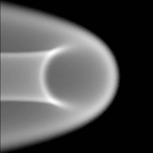
camera = PinholeCamera((256, 256), pipelines=[PowerPipeline2D()], parent=world)
camera.transform = translate(2.5, -4.5, 0)*rotate_basis(Vector3D(0, 1, 0), Vector3D(0, 0, 1))
camera.pixel_samples = 1
plt.ion()
camera.observe()
plt.ioff()
plt.show()
# Copyright 2016-2018 Euratom
# Copyright 2016-2018 United Kingdom Atomic Energy Authority
# Copyright 2016-2018 Centro de Investigaciones Energéticas, Medioambientales y Tecnológicas
#
# Licensed under the EUPL, Version 1.1 or – as soon they will be approved by the
# European Commission - subsequent versions of the EUPL (the "Licence");
# You may not use this work except in compliance with the Licence.
# You may obtain a copy of the Licence at:
#
# https://joinup.ec.europa.eu/software/page/eupl5
#
# Unless required by applicable law or agreed to in writing, software distributed
# under the Licence is distributed on an "AS IS" basis, WITHOUT WARRANTIES OR
# CONDITIONS OF ANY KIND, either express or implied.
#
# See the Licence for the specific language governing permissions and limitations
# under the Licence.


import numpy as np
import matplotlib.pyplot as plt
from scipy.constants import electron_mass, atomic_mass

from raysect.core.math.function.float import Arg2D, Exp2D, Sqrt2D
from raysect.primitive import Cylinder
from raysect.optical import World, translate, Point3D, Vector3D, rotate_basis, Spectrum
from raysect.optical.observer import PinholeCamera, PowerPipeline2D

from cherab.core import Species, Maxwellian, Plasma, Line
from cherab.core.math import sample3d, AxisymmetricMapper
from cherab.core.atomic import deuterium
from cherab.core.model import ExcitationLine
from cherab.openadas import OpenADAS


def NeutralFunction(peak_value, sigma, magnetic_axis, lcfs_radius=1):
    """A neutral profile that is constant outside the plasma,
       then exponentially decays inside the LCFS."""
    raxis = magnetic_axis[0]
    zaxis = magnetic_axis[1]
    radius_from_axis = Sqrt2D((Arg2D('x') - raxis)**2 + (Arg2D('y') - zaxis)**2)
    scale = Exp2D(-((radius_from_axis - lcfs_radius)**2) / (2 * sigma**2))
    inside_lcfs = (radius_from_axis <= lcfs_radius)
    # density = peak * scale * inside_lcfs + peak * (inside_lcfs - 1).
    # Rearrange so inside_lcfs and scale are only called once each.
    density = peak_value * (inside_lcfs * (scale - 1) + 1)
    return AxisymmetricMapper(density)


def IonFunction(v_core, v_lcfs, magnetic_axis, p=4, q=3, lcfs_radius=1):
    """An approximate toroidal plasma profile that follows a double
       quadratic between the LCFS and magnetic axis."""
    r_axis = magnetic_axis[0]
    z_axis = magnetic_axis[1]
    radius_from_axis = Sqrt2D((Arg2D('x') - r_axis)**2 + (Arg2D('y') - z_axis)**2)
    density = (v_core - v_lcfs) * (1 - (radius_from_axis / lcfs_radius)**p)**q + v_lcfs
    inside_lcfs = (radius_from_axis <= lcfs_radius)
    return AxisymmetricMapper(density * inside_lcfs)


# tunables
peak_density = 1e19
peak_temperature = 2500
magnetic_axis = (2.5, 0)


# setup scenegraph
world = World()


###################
# plasma creation #

plasma = Plasma(parent=world)
plasma.atomic_data = OpenADAS(permit_extrapolation=True)
plasma.geometry = Cylinder(3.5, 2.2, transform=translate(0, 0, -1.1))
plasma.geometry_transform = translate(0, 0, -1.1)

# No net velocity for any species
zero_velocity = Vector3D(0, 0, 0)

# define neutral species distribution
d0_density = NeutralFunction(peak_density, 0.1, magnetic_axis)
d0_temperature = 0.5  # constant 0.5eV temperature for all neutrals
d0_distribution = Maxwellian(d0_density, d0_temperature, zero_velocity,
                             deuterium.atomic_weight * atomic_mass)
d0_species = Species(deuterium, 0, d0_distribution)

# define deuterium ion species distribution
d1_density = IonFunction(peak_density, 0, magnetic_axis)
d1_temperature = IonFunction(peak_temperature, 0, magnetic_axis)
d1_distribution = Maxwellian(d1_density, d1_temperature, zero_velocity,
                             deuterium.atomic_weight * atomic_mass)
d1_species = Species(deuterium, 1, d1_distribution)

# define the electron distribution
e_density = IonFunction(peak_density, 0, magnetic_axis)
e_temperature = IonFunction(peak_temperature, 0, magnetic_axis)
e_distribution = Maxwellian(e_density, e_temperature, zero_velocity, electron_mass)

# define species
plasma.b_field = Vector3D(1.0, 1.0, 1.0)
plasma.electron_distribution = e_distribution
plasma.composition = [d0_species, d1_species]

# Add a balmer alpha line for visualisation purposes
d_alpha_excit = ExcitationLine(Line(deuterium, 0, (3, 2)))
plasma.models = [d_alpha_excit]


####################
# Visualise Plasma #

# Run some plots to check the distribution functions and emission profile are as expected
r, _, z, t_samples = sample3d(d1_temperature, (0, 4, 200), (0, 0, 1), (-2, 2, 200))
plt.imshow(np.transpose(np.squeeze(t_samples)), extent=[0, 4, -2, 2])
plt.colorbar()
plt.axis('equal')
plt.xlabel('r axis')
plt.ylabel('z axis')
plt.title("Ion temperature profile in r-z plane")

plt.figure()
r, _, z, t_samples = sample3d(d1_temperature, (-4, 4, 400), (-4, 4, 400), (0, 0, 1))
plt.imshow(np.transpose(np.squeeze(t_samples)), extent=[-4, 4, -4, 4])
plt.colorbar()
plt.axis('equal')
plt.xlabel('x axis')
plt.ylabel('y axis')
plt.title("Ion temperature profile in x-y plane")

plt.figure()
r, _, z, t_samples = sample3d(d0_density, (0, 4, 200), (0, 0, 1), (-2, 2, 200))
plt.imshow(np.transpose(np.squeeze(t_samples)), extent=[0, 4, -2, 2])
plt.colorbar()
plt.axis('equal')
plt.xlabel('r axis')
plt.ylabel('z axis')
plt.title("Neutral Density profile in r-z plane")

plt.figure()
xrange = np.linspace(0, 4, 200)
yrange = np.linspace(-2, 2, 200)
d_alpha_rz_intensity = np.zeros((200, 200))
direction = Vector3D(0, 1, 0)
for i, x in enumerate(xrange):
    for j, y in enumerate(yrange):
        emission = d_alpha_excit.emission(Point3D(x, 0.0, y), direction, Spectrum(650, 660, 1))
        d_alpha_rz_intensity[j, i] = emission.total()
plt.imshow(d_alpha_rz_intensity, extent=[0, 4, -2, 2], origin='lower')
plt.colorbar()
plt.xlabel('r axis')
plt.ylabel('z axis')
plt.title("D-alpha emission in R-Z")


camera = PinholeCamera((256, 256), pipelines=[PowerPipeline2D()], parent=world)
camera.transform = translate(2.5, -4.5, 0)*rotate_basis(Vector3D(0, 1, 0), Vector3D(0, 0, 1))
camera.pixel_samples = 1

plt.ion()
camera.observe()
plt.ioff()
plt.show()