Zeeman Spectroscopy
In the presence of magnetic field, spectral lines split into several components. For high-resolution spectroscopy in magnetic confinement devices, Zeeman effect must be taken into account. Ususally, Zeeman effect is used in plasma diagnostics to determine spatial location of the radiation source, namely high-field side scrape-off layer versus low-field side scrape-off layer.
Different Zeeman components have different polarisations, so-called \(\pi\)- and \(\sigma\)-polarised components. Therefore, the observed spectrum depends on the angle between the direction of observation and the magnetic field. When observed along the magnetic field direction, only \(\sigma\)-polarised components are visible.
Cherab contains the following models of Zeeman line shapes.
ZeemanTripletmodel can be used in the case when the magnetic field is strong enough to disrupt the coupling between orbital and spin angular momenta of the electron (Paschen–Back effect).ParametrisedZeemanTripletshould be used when the Paschen–Back effect is stil observed, but the broadening due to the line’s fine structure cannot be ignored. See A. Blom and C. Jupén, Parametrisation of the Zeeman effect for hydrogen-like spectra in high-temperature plasmas, Plasma Phys. Control. Fusion 44 (2002) 1229-1241.In all other cases, the general
ZeemanMultipletmodel must be used. The input data for this model can be obtained with the ADAS603 subroutines.
In case of \(D_{\alpha}\) spectral line, all three models give the same results. This demo shows how the spectrum depends on the angle between the direction of observation and the magnetic field.
# Copyright 2016-2018 Euratom
# Copyright 2016-2018 United Kingdom Atomic Energy Authority
# Copyright 2016-2018 Centro de Investigaciones Energéticas, Medioambientales y Tecnológicas
#
# Licensed under the EUPL, Version 1.1 or – as soon they will be approved by the
# European Commission - subsequent versions of the EUPL (the "Licence");
# You may not use this work except in compliance with the Licence.
# You may obtain a copy of the Licence at:
#
# https://joinup.ec.europa.eu/software/page/eupl5
#
# Unless required by applicable law or agreed to in writing, software distributed
# under the Licence is distributed on an "AS IS" basis, WITHOUT WARRANTIES OR
# CONDITIONS OF ANY KIND, either express or implied.
#
# See the Licence for the specific language governing permissions and limitations
# under the Licence.


# External imports
from numpy import cos, sin, deg2rad
import matplotlib.pyplot as plt
from scipy.constants import electron_mass, atomic_mass
from raysect.core.math.function.float import Arg1D, Constant1D
from raysect.optical import World, Vector3D, Point3D, Ray
from raysect.primitive import Sphere
from raysect.optical.material.emitter.inhomogeneous import NumericalIntegrator

# Cherab imports
from cherab.core import Species, Maxwellian, Plasma, Line
from cherab.core.atomic import ZeemanStructure
from cherab.core.atomic.elements import deuterium
from cherab.core.model import ExcitationLine, RecombinationLine, ZeemanTriplet, ParametrisedZeemanTriplet, ZeemanMultiplet
from cherab.openadas import OpenADAS
from cherab.tools.plasmas import GaussianVolume


# tunables
ion_density = 1e19
sigma = 0.25

# setup scenegraph
world = World()

# create atomic data source
adas = OpenADAS(permit_extrapolation=True)

# PLASMA ----------------------------------------------------------------------
plasma = Plasma(parent=world)
plasma.atomic_data = adas
plasma.geometry = Sphere(sigma * 5.0)
plasma.geometry_transform = None
plasma.integrator = NumericalIntegrator(step=sigma / 5.0)

# define basic distributions
d_density = GaussianVolume(0.5 * ion_density, sigma * 10000)
e_density = GaussianVolume(ion_density, sigma * 10000)
temperature = 1 + GaussianVolume(79, sigma)
bulk_velocity = Vector3D(0, 0, 0)

deuterium_mass = deuterium.atomic_weight * atomic_mass
d0_distribution = Maxwellian(d_density, 0.5 * temperature, bulk_velocity, deuterium_mass)
d1_distribution = Maxwellian(d_density, temperature, bulk_velocity, deuterium_mass)
e_distribution = Maxwellian(e_density, temperature, bulk_velocity, electron_mass)

d0_species = Species(deuterium, 0, d0_distribution)
d1_species = Species(deuterium, 1, d1_distribution)

# define magnetic field
plasma.b_field = Vector3D(0, 0, 6.0)

# define species
plasma.electron_distribution = e_distribution
plasma.composition = [d0_species, d1_species]

# setup D-alpha line
deuterium_I_656 = Line(deuterium, 0, (3, 2))  # n = 3->2: 656.1nm

# add simple Zeeman triplet model to the plasma
plasma.models = [
    ExcitationLine(deuterium_I_656, lineshape=ZeemanTriplet),
    RecombinationLine(deuterium_I_656, lineshape=ZeemanTriplet)
]

# angles between the ray and the magnetic field direction
angles = (0., 45., 90.)

# Ray-trace the spectrum for different angles between the ray and the magnetic field
triplet = []
for angle in angles:
    angle_rad = deg2rad(angle)
    r = Ray(origin=Point3D(0, -5 * sin(angle_rad), -5 * cos(angle_rad)), direction=Vector3D(0, sin(angle_rad), cos(angle_rad)),
            min_wavelength=655.4, max_wavelength=656.8, bins=500)
    triplet.append(r.trace(world))

# add parametrised Zeeman triplet model to the plasma
# this model taeks into account additional broadening due to the line's fine structure
# without resolving the individual components of the fine structure
plasma.models = [
    ExcitationLine(deuterium_I_656, lineshape=ParametrisedZeemanTriplet),
    RecombinationLine(deuterium_I_656, lineshape=ParametrisedZeemanTriplet)
]

# Ray-trace the spectrum again
parametrised_triplet = []
for angle in angles:
    angle_rad = deg2rad(angle)
    r = Ray(origin=Point3D(0, -5 * sin(angle_rad), -5 * cos(angle_rad)), direction=Vector3D(0, sin(angle_rad), cos(angle_rad)),
            min_wavelength=655.4, max_wavelength=656.8, bins=500)
    parametrised_triplet.append(r.trace(world))

# add ZeemanMultiplet model to the plasma

# initialising the splitting function
BOHR_MAGNETON = 5.78838180123e-5  # in eV/T
HC_EV_NM = 1239.8419738620933  # (Planck constant in eV s) x (speed of light in nm/s)
wavelength = plasma.atomic_data.wavelength(deuterium, 0, (3, 2))
photon_energy = HC_EV_NM / wavelength

pi_components = [(Constant1D(wavelength), Constant1D(1.0))]
sigma_minus_components = [(HC_EV_NM / (photon_energy - BOHR_MAGNETON * Arg1D()), Constant1D(0.5))]
sigma_plus_components = [(HC_EV_NM / (photon_energy + BOHR_MAGNETON * Arg1D()), Constant1D(0.5))]

zeeman_structure = ZeemanStructure(pi_components, sigma_plus_components, sigma_minus_components)

plasma.models = [
    ExcitationLine(deuterium_I_656, lineshape=ZeemanMultiplet, lineshape_args=[zeeman_structure]),
    RecombinationLine(deuterium_I_656, lineshape=ZeemanMultiplet, lineshape_args=[zeeman_structure])
]

# Ray-trace the spectrum again
multiplet = []
for angle in angles:
    angle_rad = deg2rad(angle)
    r = Ray(origin=Point3D(0, -5 * sin(angle_rad), -5 * cos(angle_rad)), direction=Vector3D(0, sin(angle_rad), cos(angle_rad)),
            min_wavelength=655.4, max_wavelength=656.8, bins=500)
    multiplet.append(r.trace(world))

for i, angle in enumerate(angles):
    plt.figure()
    plt.plot(triplet[i].wavelengths, triplet[i].samples, ls='-', label='ZeemanTriplet')
    plt.plot(parametrised_triplet[i].wavelengths, parametrised_triplet[i].samples, ls='--', label='ParametrisedZeemanTriplet')
    plt.plot(multiplet[i].wavelengths, multiplet[i].samples, ls=':', label='ZeemanMultiplet')
    plt.legend()
    plt.xlabel('Wavelength (nm)')
    plt.ylabel('Radiance (W/m^2/str/nm)')
    plt.title(r'Observed spectrum at {}$\degree$ angle between ray and magnetic field'.format(angle))
plt.show()
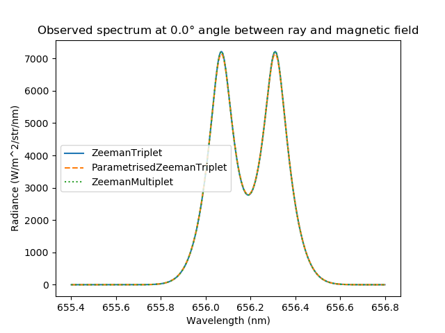
Caption: The \(D_{\alpha}\) spectrum observed along the magnetic field.
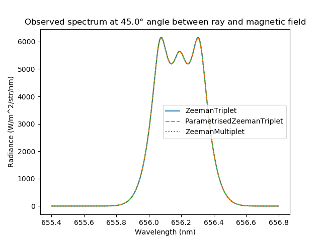
Caption: The \(D_{\alpha}\) spectrum observed at \(45^{\circ}\) angle between the direction of ray and the magnetic field.
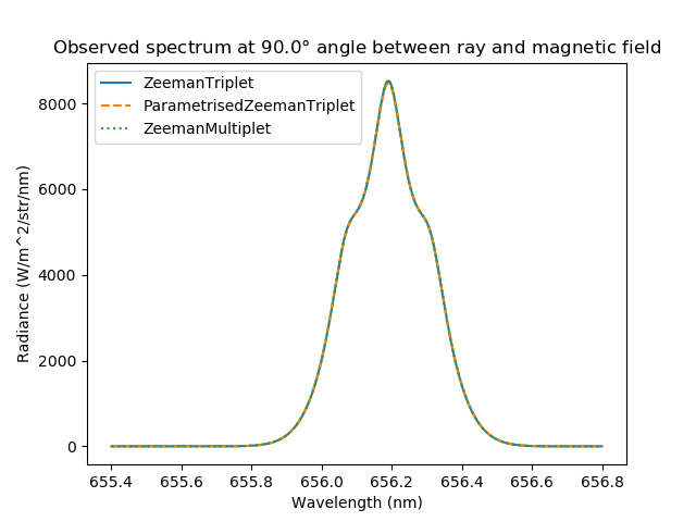
Caption: The \(D_{\alpha}\) spectrum observed perpendicularly to the magnetic field.