Stark Broadening

Normally, the dominant factor in determining the lineshape is the thermal doppler broadening. However, in certain high density plasma scenarios a secondary effect can take over, known as pressure broadening. This effect results from the fact that radiating ions experience a change in the electric field due to the presence of neighbouring ions. In normal tokamak operations this effect is negligible, except in the divertor region.

It is possible to override the default doppler broadened line shape by specifying the StarkBroadenedLine() lineshape class. In this example we can see two stark broadened balmer series lines surrounding a Nitrogen II multiplet feature.

# Copyright 2016-2018 Euratom
# Copyright 2016-2018 United Kingdom Atomic Energy Authority
# Copyright 2016-2018 Centro de Investigaciones Energéticas, Medioambientales y Tecnológicas
#
# Licensed under the EUPL, Version 1.1 or – as soon they will be approved by the
# European Commission - subsequent versions of the EUPL (the "Licence");
# You may not use this work except in compliance with the Licence.
# You may obtain a copy of the Licence at:
#
# https://joinup.ec.europa.eu/software/page/eupl5
#
# Unless required by applicable law or agreed to in writing, software distributed
# under the Licence is distributed on an "AS IS" basis, WITHOUT WARRANTIES OR
# CONDITIONS OF ANY KIND, either express or implied.
#
# See the Licence for the specific language governing permissions and limitations
# under the Licence.


# External imports
import matplotlib.pyplot as plt
from scipy.constants import electron_mass, atomic_mass
from raysect.optical import World, translate, rotate, Vector3D, Point3D, Ray
from raysect.primitive import Sphere
from raysect.optical.material.emitter.inhomogeneous import NumericalIntegrator

# Cherab imports
from cherab.core import Species, Maxwellian, Plasma, Line
from cherab.core.atomic.elements import deuterium, nitrogen
from cherab.core.model import ExcitationLine, RecombinationLine,\
    MultipletLineShape, StarkBroadenedLine
from cherab.openadas import OpenADAS
from cherab.tools.plasmas import GaussianVolume


# tunables
ion_density = 1e20
sigma = 0.25

# setup scenegraph
world = World()

# create atomic data source
adas = OpenADAS(permit_extrapolation=True)

# PLASMA ----------------------------------------------------------------------
plasma = Plasma(parent=world)
plasma.atomic_data = adas
plasma.geometry = Sphere(sigma * 5.0)
plasma.geometry_transform = None
plasma.integrator = NumericalIntegrator(step=sigma / 5.0)

# define basic distributions
d_density = GaussianVolume(0.5 * ion_density, sigma*10000)
n_density = d_density * 0.01
e_density = GaussianVolume(ion_density, sigma*10000)
temperature = 1 + GaussianVolume(79, sigma)
bulk_velocity = Vector3D(-1e6, 0, 0)

deuterium_mass = deuterium.atomic_weight * atomic_mass
d_distribution = Maxwellian(d_density, temperature, bulk_velocity, deuterium_mass)
nitrogen_mass = nitrogen.atomic_weight * atomic_mass
n_distribution = Maxwellian(n_density, temperature, bulk_velocity, nitrogen_mass)
e_distribution = Maxwellian(e_density, temperature, bulk_velocity, electron_mass)

d0_species = Species(deuterium, 0, d_distribution)
d1_species = Species(deuterium, 1, d_distribution)
n1_species = Species(nitrogen, 1, n_distribution)

# define species
plasma.b_field = Vector3D(1.0, 1.0, 1.0)
plasma.electron_distribution = e_distribution
plasma.composition = [d0_species, d1_species, n1_species]

# setup the Balmer lines
hydrogen_I_410 = Line(deuterium, 0, (6, 2))  # n = 6->2: 410.12nm
hydrogen_I_396 = Line(deuterium, 0, (7, 2))  # n = 7->2: 396.95nm

# setup the Nitrgon II line with multiplet splitting instructions
nitrogen_II_404 = Line(nitrogen, 1, ("2s2 2p1 4f1 3G13.0", "2s2 2p1 3d1 3F10.0"))
multiplet = [[403.509, 404.132, 404.354, 404.479, 405.692],
             [0.205, 0.562, 0.175, 0.029, 0.029]]

# add all lines to the plasma
plasma.models = [
    ExcitationLine(hydrogen_I_410, lineshape=StarkBroadenedLine),
    RecombinationLine(hydrogen_I_410, lineshape=StarkBroadenedLine),
    ExcitationLine(hydrogen_I_396, lineshape=StarkBroadenedLine),
    RecombinationLine(hydrogen_I_396, lineshape=StarkBroadenedLine),
    ExcitationLine(nitrogen_II_404, lineshape=MultipletLineShape, lineshape_args=[multiplet]),
]


# Ray-trace and plot the results
r = Ray(origin=Point3D(0, 0, -5), direction=Vector3D(0, 0, 1),
        min_wavelength=395, max_wavelength=415, bins=2000)
s = r.trace(world)
plt.plot(s.wavelengths, s.samples)
plt.xlabel('Wavelength (nm)')
plt.ylabel('Radiance (W/m^2/str/nm)')
plt.title('Observed Spectrum')
plt.show()

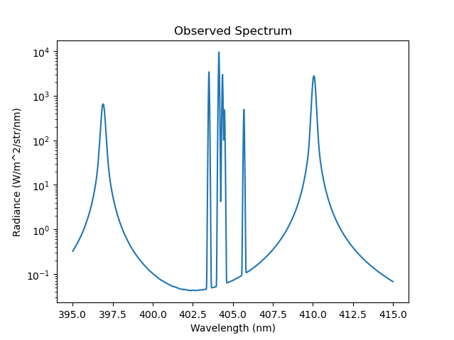
Caption: The observed spectrum with two stark broadened balmer lines (397nm and 410nm) surrounding a NII multiplet feature.

Caption: A zoomed in view of the 410nm Balmer line revealing the characteristic stark broadened lineshape.