Impact Excitation and Recombination

This demonstration shows how to model the commonly observed passive emission lines due to electron impact excitation and recombination. A spherical plasma is initialised in a similar way to other demonstrations on creating plasmas. Then the ExcitationLine() and RecombinationLine() emission models for the first five Balmer series lines are attached to the plasma.

# Copyright 2016-2018 Euratom
# Copyright 2016-2018 United Kingdom Atomic Energy Authority
# Copyright 2016-2018 Centro de Investigaciones Energéticas, Medioambientales y Tecnológicas
#
# Licensed under the EUPL, Version 1.1 or – as soon they will be approved by the
# European Commission - subsequent versions of the EUPL (the "Licence");
# You may not use this work except in compliance with the Licence.
# You may obtain a copy of the Licence at:
#
# https://joinup.ec.europa.eu/software/page/eupl5
#
# Unless required by applicable law or agreed to in writing, software distributed
# under the Licence is distributed on an "AS IS" basis, WITHOUT WARRANTIES OR
# CONDITIONS OF ANY KIND, either express or implied.
#
# See the Licence for the specific language governing permissions and limitations
# under the Licence.


# External imports
import os
from scipy.constants import electron_mass, atomic_mass

import matplotlib.pyplot as plt
import numpy as np
from cherab.core.model import ExcitationLine, RecombinationLine, Bremsstrahlung

# Cherab and raysect imports
from cherab.core import Species, Maxwellian, Plasma, Line, elements
from cherab.openadas import OpenADAS
from cherab.tools.plasmas import GaussianVolume

# Core and external imports
from raysect.optical import World, translate, rotate, Vector3D, Point3D, Ray
from raysect.primitive import Sphere
from raysect.optical.observer import PinholeCamera
from raysect.optical.material.emitter.inhomogeneous import NumericalIntegrator

# tunables
ion_density = 1e19
sigma = 0.25

# setup scenegraph
world = World()

# create atomic data source
adas = OpenADAS(permit_extrapolation=True)

# PLASMA ----------------------------------------------------------------------
plasma = Plasma(parent=world)
plasma.atomic_data = adas
plasma.geometry = Sphere(sigma * 5.0)
plasma.geometry_transform = None
plasma.integrator = NumericalIntegrator(step=sigma / 5.0)

# define basic distributions
d_density = GaussianVolume(0.5 * ion_density, sigma*10000)
e_density = GaussianVolume(ion_density, sigma*10000)
temperature = 1 + GaussianVolume(79, sigma)
bulk_velocity = Vector3D(-1e5, 0, 0)

d_mass = elements.deuterium.atomic_weight * atomic_mass
d_distribution = Maxwellian(d_density, temperature, bulk_velocity, d_mass)
e_distribution = Maxwellian(e_density, temperature, bulk_velocity, electron_mass)

d0_species = Species(elements.deuterium, 0, d_distribution)
d1_species = Species(elements.deuterium, 1, d_distribution)

# define species
plasma.b_field = Vector3D(1.0, 1.0, 1.0)
plasma.electron_distribution = e_distribution
plasma.composition = [d0_species, d1_species]

# Setup elements.deuterium lines
d_alpha = Line(elements.deuterium, 0, (3, 2))
d_beta = Line(elements.deuterium, 0, (4, 2))
d_gamma = Line(elements.deuterium, 0, (5, 2))
d_delta = Line(elements.deuterium, 0, (6, 2))
d_epsilon = Line(elements.deuterium, 0, (7, 2))

plasma.models = [
    Bremsstrahlung(),
    ExcitationLine(d_alpha),
    ExcitationLine(d_beta),
    ExcitationLine(d_gamma),
    ExcitationLine(d_delta),
    ExcitationLine(d_epsilon),
    RecombinationLine(d_alpha),
    RecombinationLine(d_beta),
    RecombinationLine(d_gamma),
    RecombinationLine(d_delta),
    RecombinationLine(d_epsilon)
]


plt.ion()

r = Ray(origin=Point3D(0, 0, -5), direction=Vector3D(0, 0, 1),
        min_wavelength=100, max_wavelength=1000, bins=1e6)
s = r.trace(world)
plt.plot(s.wavelengths, s.samples)

r = Ray(origin=Point3D(-5, 0, -5), direction=Vector3D(1, 0, 1),
        min_wavelength=100, max_wavelength=1000, bins=1e6)
s = r.trace(world)
plt.plot(s.wavelengths, s.samples)

r = Ray(origin=Point3D(-5, 0, 0), direction=Vector3D(1, 0, 0),
        min_wavelength=100, max_wavelength=1000, bins=1e6)
s = r.trace(world)
plt.plot(s.wavelengths, s.samples)

plt.xlabel('Wavelength (nm)')
plt.ylabel('Radiance (W/m^2/str/nm)')
plt.title('Sampled Balmer Series Spectrum')
plt.show()

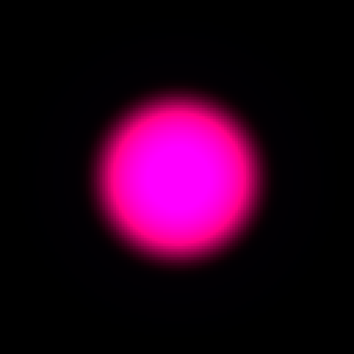
camera = PinholeCamera((128, 128), parent=world, transform=translate(0, 0, -3.5))
camera.spectral_rays = 1
camera.spectral_bins = 15
camera.pixel_samples = 50

plt.ion()
camera.observe()

plt.ioff()
plt.show()

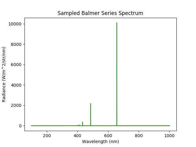
Caption: The observed Balmer series spectrum.

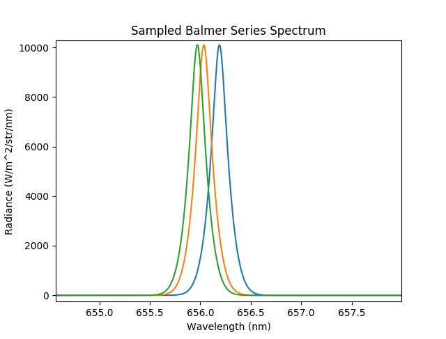
Caption: A zoomed in view on the h-alpha lines reveals the doppler shifts observable by varying the viewing angle.

Caption: A zoomed in spectral view of the commonly studied CVI n = 8->7 CXS line. The lines are doppler shifted due to the velocity of the plasma.