Custom emission model
Example of how to make a custom electron impact excitation emission model. A MAST-U SOLPS plasma simulation will be used to drive the emission model. The full demo file for this tutorial can be downloaded from here. Start by importing all required modules and creating world.
# Core and external imports
from pylab import ion
from math import sqrt, exp
from scipy.constants import elementary_charge, speed_of_light, pi

from raysect.optical import World, translate
from raysect.optical.observer.vector_camera import VectorCamera
from raysect.primitive import Cylinder, import_stl
from raysect.optical.material.absorber import AbsorbingSurface
from raysect.optical.material.emitter import VolumeEmitterInhomogeneous

# Cherab and raysect imports
from cherab.atomic.core import Line
from cherab.atomic.elements import deuterium
from cherab.atomic.adas.adf_files.read_adf15 import get_adf15_pec
from cherab_contrib.jet.calcam import load_calcam_calibration
from cherab_contrib.simulation_data.solps.solps_plasma import SOLPSSimulation


# Define constants
PI = pi
AMU = 1.66053892e-27
ELEMENTARY_CHARGE = elementary_charge
SPEED_OF_LIGHT = speed_of_light

world = World()
Loading Plasma and machine geometry
Load all parts of the machine mesh from files (either .stl or .obj). Each CAD files’ optical properties are modified by the chosen material. In this case an AbsorbingSurface is being used, which acts like a perfect absorber. This class is useful for using the mesh geometry to restrict the plasma view, without including more advanced behaviour such as reflections.
MESH_PARTS = ['/projects/cadmesh/mast/mastu-light/mug_centrecolumn_endplates.stl',
              '/projects/cadmesh/mast/mastu-light/mug_divertor_nose_plates.stl']

for path in MESH_PARTS:
    import_stl(path, parent=world, material=AbsorbingSurface())  # Mesh with perfect absorber
The core Plasma object will be populated from the output of a SOLPS simulation. This example loads a SOLPS simulation from the AUG server.
# Load plasma from SOLPS model
mds_server = 'solps-mdsplus.aug.ipp.mpg.de:8001'
ref_number = 69636
sim = SOLPSSimulation.load_from_mdsplus(mds_server, ref_number)
plasma = sim.plasma
mesh = sim.mesh
vessel = mesh.vessel
Custom emission model
Custom emitters are implemented as Raysect materials with the VolumeEmitterInhomogeneous class. You model should inherit from this base class, only two methods need to be implemented, the __init__() and emission_function() methods.
The __init__() method should be used to setup any plasma parameters you will need access to for calculations. You could pass in the whole plasma object, or alternatively just the species you need. In this example, I will need the electron distribution and atomic deuterium distribution. Both of these can be passed in from the plasma object.
I’m also passing in a spectroscopic Line object which holds useful information about my emission line. But this can change alot from application to application. We are also loading some atomic data from ADAS. You could optionally pass in the atomic data you want to use in the __init__().
The step parameter is the only parameter required by the parent VolumeEmitterInhomogeneous class. This parameter determines the integration step size for sampling and will need to be adjusted based on your application’s scale lengths. Make ure you call the parent init whith the super method, e.g. super().__init__(step=step).
All the magic happens in the emission_function() method. This method is called at every point in space where the ray-tracer would like to know the emission. The arguments are fixed and are as follows:
point (Point3D) - current position in local primitive coordinates
direction (Vector3D) - current ray direction in local primitive coordinates
spectrum (Spectrum) - measured spectrum so far. Don’t overwrite it. Add your local emission to the measured spectrum. Units are in spectral radiance (W/m3/str/nm).
world (World) - the world being ray-traced. You may have multiple worlds.
ray (Ray) - the current ray being traced.
primitive (Primitive) - the primitive container for this material. Could be a sphere, cyliner, or CAD mesh for example.
to_local (AffineMatrix3D) - Affine matrix for coordinate transformations to local coordinates.
to_world (AffineMatrix3D) - Affine matrix for coordinate transformations to world coordinates.
Here is an example class implementation of an excitation line.
class ExcitationLine(VolumeEmitterInhomogeneous):

    def __init__(self, line, electron_distribution, atom_species, step=0.005,
                 block=0, filename=None):

        super().__init__(step=step)

        self.line = line
        self.electron_distribution = electron_distribution
        self.atom_species = atom_species

        # Function to load ADAS rate coefficients
        # Replace this with your own atomic data as necessary.
        self.pec_excitation = get_adf15_pec(line, 'EXCIT', filename=filename, block=block)

    def emission_function(self, point, direction, spectrum, world, ray, primitive,
                          to_local, to_world):

        ##########################################
        # Load all data you need for calculation #

        # Get the current position in world coordinates,
        # 'point' is in local primitive coordinates by default
        x, y, z = point.transform(to_world)

        # electron density n_e(x, y, z) at current point
        ne = self.electron_distribution.density(x, y, z)
        # electron temperature t_e(x, y, z) at current point
        te = self.electron_distribution.effective_temperature(x, y, z)
        # density of neutral atoms of species specified by line.element
        na = self.atom_species.distribution.density(x, y, z)

        # Electron temperature and density must be in valid range for ADAS data.
        if not 5E13 < ne < 2E21:
            return spectrum
        if not 0.2 < te < 10000:
            return spectrum

        # Photo Emission Coefficient (PEC) for excitation at this temperature and density
        pece = self.pec_excitation(ne, te)

        # calculate line intensity
        inty = 1E6 * (pece * ne * na)  # 1E6 factor because ADAS units are in cm^-3

        weight = self.line.element.atomic_weight
        rest_wavelength = self.line.wavelength

        ###############################
        # Calculate the emission line #

        # Calculate a simple gaussian line at each line wavelength in spectrum
        # Add it to the existing spectrum. Don't override previous results!

        sigma = sqrt(te * ELEMENTARY_CHARGE / (weight * AMU)) * rest_wavelength / SPEED_OF_LIGHT
        i0 = inty/(sigma * sqrt(2 * PI))
        width = 2*sigma**2
        for i, wvl in enumerate(spectrum.wavelengths):
            spectrum.samples[i] += i0 * exp(-(wvl - rest_wavelength)**2 / width)

        return spectrum
Once you have an emission model, initialise the class and populate its attributes.
# Setup deuterium line
d_alpha = Line(deuterium, 0, (3, 2), wavelength=656.19)

# Load the deuterium atom species and electron distribution for use in rate calculations.
d_atom_species = plasma.get_species(deuterium, 0)
electrons = plasma.electron_distribution

# Load the Excitation and Recombination lines and add them as emitters to the world.
d_alpha_excit = ExcitationLine(d_alpha, plasma.electron_distribution, d_atom_species)
All materials need to be attached to some geometry, in this case we attach our emission model to a cylinder with the approximate vessel geometry.
outer_radius = plasma.misc_properties['maxr'] + 0.001
plasma_height = plasma.misc_properties['maxz'] - plasma.misc_properties['minz']
lower_z = plasma.misc_properties['minz']

main_plasma_cylinder = Cylinder(outer_radius, plasma_height, parent=world,
                                material=d_alpha_excit, transform=translate(0, 0, lower_z))
Camera setup
Setup an example MAST-U camera with Calcam and VectorCamera.
# Load a MAST-U midplane camera
camera_config = load_calcam_calibration('./demo/mast/camera_configs/mug_bulletb_midplane.nc')

# Setup camera for interactive use...
pixels_shape, pixel_origins, pixel_directions = camera_config
camera = VectorCamera(pixel_origins, pixel_directions, parent=world)
camera.spectral_bins = 15
camera.pixel_samples = 1
ion()
camera.observe()
Example output images
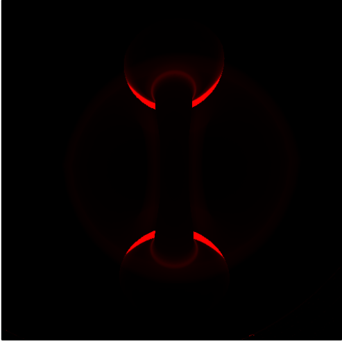
D-alpha with the mid-plane bullet camera. This example combines excitation and recombination rates. Divertor recombination dominates when line integration is taking into account.