Measuring line of sight spectra

Cherab is capable of simulating spectroscopic measurements. In this example we simulate a basic measurement of the balmer series in the MAST-U divertor with an optical fibre.

By default, Raysect images are ray-traced to give line integrated spectra which can sometimes be difficult to interpret without knowing the localisation of the emission. Sometimes the emission can be highly localised, and other times very diffuse. This example also shows some techniques for visualising the emission locations and plasma parameters along the ray trajectory. The full demo file for this tutorial can be downloaded from here. Start by importing all required modules and creating world.

# External imports
import os
import numpy as np
import matplotlib.pyplot as plt

# Core and external imports
from raysect.core import Vector3D, Point3D
from raysect.core.ray import Ray as CoreRay
from raysect.primitive.mesh import Mesh, import_stl
from raysect.optical.material.absorber import AbsorbingSurface
from raysect.optical.observer import FibreOptic, SpectralPipeline0D
from raysect.optical import World, translate, rotate, rotate_basis

# Cherab and raysect imports
from cherab.atomic.core import Line
from cherab.atomic.elements import deuterium, carbon
from cherab_contrib.simulation_data.solps.solps_plasma import SOLPSSimulation
from cherab.model.impact_excitation.pec_line import ExcitationLine, RecombinationLine
from cherab_mastu.mast_cad_files import CENTRE_COLUMN, LOWER_DIVERTOR_ARMOUR


plt.ion()
world = World()

Loading Plasma and machine geometry

Load all parts of the machine mesh from files. In this example we only need the centre column and divertor.

MESH_PARTS = CENTRE_COLUMN + LOWER_DIVERTOR_ARMOUR

for cad_file in MESH_PARTS:
    directory, filename = os.path.split(cad_file)
    name, ext = filename.split('.')
    print("importing {} ...".format(filename))
    Mesh.from_file(cad_file, parent=world, material=AbsorbingSurface(), name=name)

The core Plasma object will be populated from the output of a MAST-U SOLPS simulation.

# Load plasma from SOLPS model
mds_server = 'solps-mdsplus.aug.ipp.mpg.de:8001'
ref_number = 69636
sim = SOLPSSimulation.load_from_mdsplus(mds_server, ref_number)
plasma = sim.plasma
mesh = sim.mesh
vessel = mesh.vessel

We will some lines from the Balmer series in our divertor example. These lines are explained in another tutorial.

# Setup deuterium lines
d_alpha = Line(deuterium, 0, (3, 2), wavelength=656.19)
d_beta = Line(deuterium, 0, (4, 2), wavelength=486.1)
d_gamma = Line(deuterium, 0, (5, 2), wavelength=433.99)
d_delta = Line(deuterium, 0, (6, 2), wavelength=410.2)
d_epsilon = Line(deuterium, 0, (7, 2), wavelength=397)

d_ion_species = plasma.get_species(deuterium, 1)
d_atom_species = plasma.get_species(deuterium, 0)

d_alpha_excit = ExcitationLine(d_alpha, plasma.electron_distribution, d_atom_species, inside_outside=plasma.inside_outside)
d_alpha_excit.add_emitter_to_world(world, plasma)
d_alpha_recom = RecombinationLine(d_alpha, plasma.electron_distribution, d_ion_species, inside_outside=plasma.inside_outside)
d_alpha_recom.add_emitter_to_world(world, plasma)

d_gamma_excit = ExcitationLine(d_gamma, plasma.electron_distribution, d_atom_species, inside_outside=plasma.inside_outside)
d_gamma_excit.add_emitter_to_world(world, plasma)
d_gamma_recom = RecombinationLine(d_gamma, plasma.electron_distribution, d_ion_species, inside_outside=plasma.inside_outside)
d_gamma_recom.add_emitter_to_world(world, plasma)

d_beta_excit = ExcitationLine(d_beta, plasma.electron_distribution, d_atom_species, inside_outside=plasma.inside_outside)
d_beta_excit.add_emitter_to_world(world, plasma)
d_beta_recom = RecombinationLine(d_beta, plasma.electron_distribution, d_ion_species, inside_outside=plasma.inside_outside)
d_beta_recom.add_emitter_to_world(world, plasma)

d_delta_excit = ExcitationLine(d_delta, plasma.electron_distribution, d_atom_species, inside_outside=plasma.inside_outside)
d_delta_excit.add_emitter_to_world(world, plasma)
d_delta_recom = RecombinationLine(d_delta, plasma.electron_distribution, d_ion_species, inside_outside=plasma.inside_outside)
d_delta_recom.add_emitter_to_world(world, plasma)

d_epsilon_excit = ExcitationLine(d_epsilon, plasma.electron_distribution, d_atom_species, inside_outside=plasma.inside_outside)
d_epsilon_excit.add_emitter_to_world(world, plasma)
d_epsilon_recom = RecombinationLine(d_epsilon, plasma.electron_distribution, d_ion_species, inside_outside=plasma.inside_outside)
d_epsilon_recom.add_emitter_to_world(world, plasma)

Optical Fibre setup

Setup an example MAST-U observation point with the FibreOptic observer class.

# Fibre position and observation direction
start_point = Point3D(1.669, 0, -1.6502)
forward_vector = Vector3D(1-1.669, 0, -2+1.6502).normalise()
up_vector = Vector3D(0, 0, 1.0)

spectra = SpectralPipeline0D()
fibre = FibreOptic([spectra], acceptance_angle=1, radius=0.001, spectral_bins=8000, spectral_rays=1,
                   pixel_samples=5, transform=translate(*start_point)*rotate_basis(forward_vector, up_vector), parent=world)

fibre.min_wavelength = 350.0
fibre.max_wavelength = 700.0

fibre.observe()

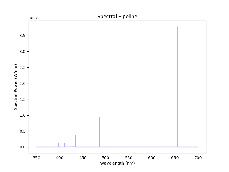
Balmer series spectrum measured with an optical fibre pointing into the MAST-U divertor.

Sampling plasma parameters along ray trajectory

The easiest way to understand the resulting spectra is to look at the predicted emission and plasma parameters along the ray trajectory. Start by finding the intersection point so that we can parameterise the ray trajectory with a parametric line equation.

# Find the next intersection point of the ray with the world
intersection = world.hit(CoreRay(start_point, forward_vector))
if intersection is not None:
    hit_point = intersection.hit_point.transform(intersection.primitive_to_world)
else:
    raise RuntimeError("No intersection with the vessel was found.")

# Traverse the ray with equation for a parametric line,
# i.e. t=0->1 traverses the ray path.
parametric_vector = start_point.vector_to(hit_point)
t_samples = np.arange(0, 1, 0.01)

Next loop over the ray positions and sample the relevant parameters.

# Setup some containers for useful parameters along the ray trajectory
ray_r_points = []
ray_z_points = []
distance = []
te = []
ne = []
dalpha = np.zeros(len(t_samples))
dgamma = np.zeros(len(t_samples))
dbeta = np.zeros(len(t_samples))
ddelta = np.zeros(len(t_samples))
depsilon = np.zeros(len(t_samples))

# get the electron distribution
electrons = plasma.electron_distribution

# At each ray position sample the parameters of interest.
for i, t in enumerate(t_samples):
    # Get new sample point location and log distance
    x = start_point.x + parametric_vector.x * t
    y = start_point.y + parametric_vector.y * t
    z = start_point.z + parametric_vector.z * t
    sample_point = Point3D(x, y, z)
    ray_r_points.append(np.sqrt(x**2 + y**2))
    ray_z_points.append(z)
    distance.append(start_point.distance_to(sample_point))

    # Sample plasma conditions
    te.append(electrons.effective_temperature(x, y, z))
    ne.append(electrons.density(x, y, z))

    # Log magnitude of emission
    dalpha[i] = d_alpha_excit.emission_at_point(x, y, z) + d_alpha_recom.emission_at_point(x, y, z)
    dgamma[i] = d_gamma_excit.emission_at_point(x, y, z) + d_gamma_recom.emission_at_point(x, y, z)
    dbeta[i] = d_beta_excit.emission_at_point(x, y, z) + d_beta_recom.emission_at_point(x, y, z)
    ddelta[i] = d_delta_excit.emission_at_point(x, y, z) + d_delta_recom.emission_at_point(x, y, z)
    depsilon[i] = d_epsilon_excit.emission_at_point(x, y, z) + d_epsilon_recom.emission_at_point(x, y, z)

Example plots

Here are some example plots that can be made with collected profiles.

# Normalise the emission arrays
dalpha /= dalpha.sum()
dgamma /= dgamma.sum()
dbeta /= dbeta.sum()
ddelta /= ddelta.sum()
depsilon /= depsilon.sum()

# Plot the trajectory parameters
sim.plot_pec_emission_lines([d_alpha_excit, d_alpha_recom], title='D_alpha')
plt.plot(ray_r_points, ray_z_points, 'k')
plt.plot(ray_r_points[0], ray_z_points[0], 'b.')
plt.plot(ray_r_points[-1], ray_z_points[-1], 'r.')

plt.figure()
plt.plot(distance, te)
plt.xlabel("Ray distance (m)")
plt.ylabel("Electron temperature (eV)")
plt.title("Electron temperature (eV) along ray path")

plt.figure()
plt.plot(distance, ne)
plt.xlabel("Ray distance (m)")
plt.ylabel("Electron density (m^-3)")
plt.title("Electron density (m^-3) along ray path")

plt.figure()
plt.plot(distance, dalpha, label='Dalpha')
plt.plot(distance, dgamma, label='Dgamma')
plt.plot(distance, dbeta, label='Dbeta')
plt.plot(distance, ddelta, label='Ddelta')
plt.plot(distance, depsilon, label='Depsilon')
plt.xlabel("Ray distance (m)")
plt.ylabel("Normalised emission")
plt.title("Normalised emission along ray path")
plt.legend()

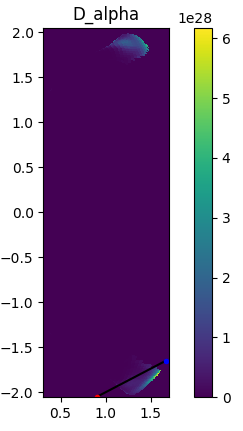
D-alpha emission in the poloidal plane. The ray trajectory is overplotted with the start and end points indicated in blue and red respectively.

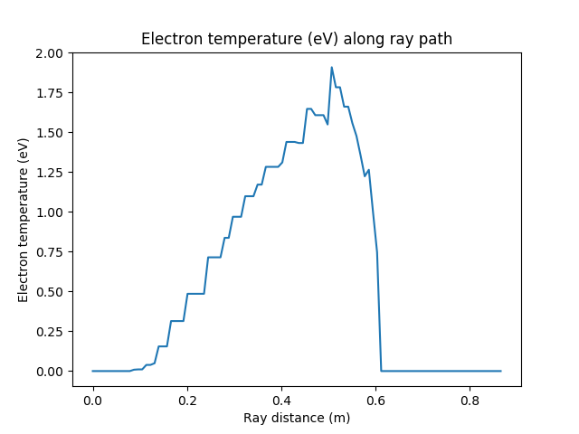
Electron temperature from the plasma sampled along the ray trajectory.

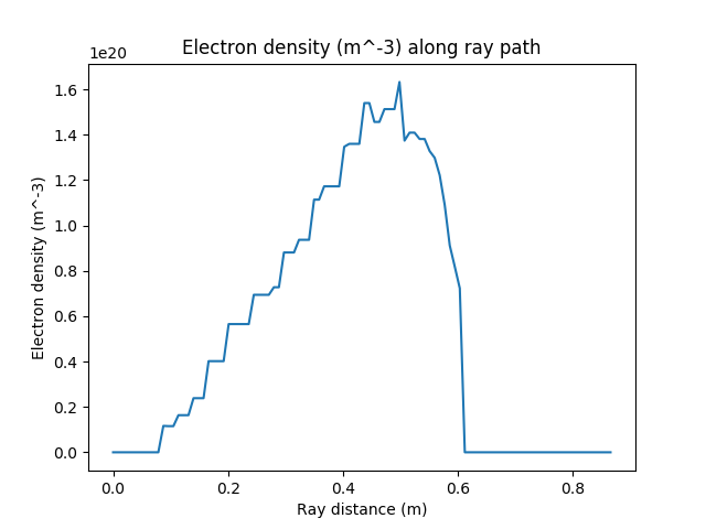
Electron density from the plasma sampled along the ray trajectory.

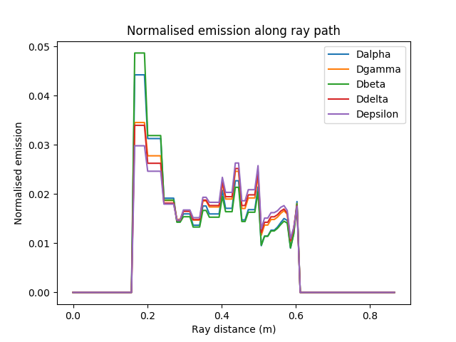
Normalised balmer series emission plotted along the ray trajectory.