Charge Exchange Spectroscopy

This demonstration shows how to model the Charge Exchange Spectroscopy (CXS) spectrum from a beam-plasma interaction. A slab plasma is setup as the target, with a neutral beam injected along the x axis. The BeamCXLine() emission model is added as a property of the beam object.

import numpy as np
import matplotlib.pyplot as plt
from scipy.constants import electron_mass, atomic_mass

from raysect.core import translate, rotate_basis, Point3D, Vector3D
from raysect.primitive import Box
from raysect.optical import World, Ray
from raysect.optical.observer import PinholeCamera

from cherab.core import Plasma, Beam, Maxwellian, Species
from cherab.core.math import sample3d, ScalarToVectorFunction3D
from cherab.core.atomic import hydrogen, deuterium, carbon, Line
from cherab.core.model import SingleRayAttenuator, BeamCXLine
from cherab.tools.plasmas.slab import NeutralFunction, IonFunction
from cherab.openadas import OpenADAS


###############
# Make Plasma #

width = 1.0
length = 1.0
height = 3.0
peak_density = 5e19
pedestal_top = 1
neutral_temperature = 0.5
peak_temperature = 2500
impurities = [(carbon, 6, 0.005)]

world = World()
adas = OpenADAS(permit_extrapolation=True, missing_rates_return_null=True)

plasma = Plasma(parent=world)
plasma.atomic_data = adas
plasma.geometry = Box(Point3D(0, -width / 2, -height / 2), Point3D(length, width / 2, height / 2))

species = []


# make a non-zero velocity profile for the plasma
vy_profile = IonFunction(1E5, 0, pedestal_top=pedestal_top)
velocity_profile = ScalarToVectorFunction3D(0, vy_profile, 0)


# define neutral species distribution
h0_density = NeutralFunction(peak_density, 0.1, pedestal_top=pedestal_top)
h0_temperature = neutral_temperature
h0_distribution = Maxwellian(h0_density, h0_temperature, velocity_profile,
                             hydrogen.atomic_weight * atomic_mass)
species.append(Species(hydrogen, 0, h0_distribution))

# define hydrogen ion species distribution
h1_density = IonFunction(peak_density, 0, pedestal_top=pedestal_top)
h1_temperature = IonFunction(peak_temperature, 0, pedestal_top=pedestal_top)
h1_distribution = Maxwellian(h1_density, h1_temperature, velocity_profile,
                             hydrogen.atomic_weight * atomic_mass)
species.append(Species(hydrogen, 1, h1_distribution))

# add impurities
if impurities:
    for impurity, ionisation, concentration in impurities:
        imp_density = IonFunction(peak_density * concentration, 0, pedestal_top=pedestal_top)
        imp_temperature = IonFunction(peak_temperature, 0, pedestal_top=pedestal_top)
        imp_distribution = Maxwellian(imp_density, imp_temperature, velocity_profile,
                                      impurity.atomic_weight * atomic_mass)
        species.append(Species(impurity, ionisation, imp_distribution))

# define the electron distribution
e_density = IonFunction(peak_density, 0, pedestal_top=pedestal_top)
e_temperature = IonFunction(peak_temperature, 0, pedestal_top=pedestal_top)
e_distribution = Maxwellian(e_density, e_temperature, velocity_profile, electron_mass)

# define species
plasma.b_field = Vector3D(0, 0, 0)
plasma.electron_distribution = e_distribution
plasma.composition = species


####################
# Visualise Plasma #

h0 = plasma.composition.get(hydrogen, 0)
h1 = plasma.composition.get(hydrogen, 1)
c6 = plasma.composition.get(carbon, 6)

# Run some plots to check the distribution functions and emission profile are as expected
h1_temp = h1.distribution.effective_temperature
r, _, z, t_samples = sample3d(h1_temp, (-1, 2, 200), (0, 0, 1), (-1, 1, 200))
plt.imshow(np.transpose(np.squeeze(t_samples)), extent=[-1, 2, -1, 1])
plt.colorbar()
plt.axis('equal')
plt.xlabel('x axis')
plt.ylabel('z axis')
plt.title("Ion temperature profile in x-z plane")

plt.figure()
r, _, z, t_samples = sample3d(h1_temp, (0, 0, 1), (-1, 1, 200), (-1, 1, 200))
plt.imshow(np.transpose(np.squeeze(t_samples)), extent=[-1, 1, -1, 1])
plt.colorbar()
plt.axis('equal')
plt.xlabel('x axis')
plt.ylabel('y axis')
plt.title("Ion temperature profile in y-z plane")

plt.figure()
h0_dens = h0.distribution.density
r, _, z, t_samples = sample3d(h0_dens, (-1, 2, 200), (0, 0, 1), (-1, 1, 200))
plt.imshow(np.transpose(np.squeeze(t_samples)), extent=[-1, 2, -1, 1])
plt.colorbar()
plt.axis('equal')
plt.xlabel('x axis')
plt.ylabel('z axis')
plt.title("Neutral Density profile in x-z plane")


###########################
# Inject beam into plasma #

cVI_8_7 = Line(carbon, 5, (8, 7))
cVI_10_8 = Line(carbon, 5, (10, 8))

integration_step = 0.0025
beam_transform = translate(-0.5, 0.0, 0) * rotate_basis(Vector3D(1, 0, 0), Vector3D(0, 0, 1))
beam_energy = 50000  # keV

beam_full = Beam(parent=world, transform=beam_transform)
beam_full.plasma = plasma
beam_full.atomic_data = adas
beam_full.energy = beam_energy
beam_full.power = 3e6
beam_full.element = deuterium
beam_full.sigma = 0.05
beam_full.divergence_x = 0.5
beam_full.divergence_y = 0.5
beam_full.length = 3.0
beam_full.attenuator = SingleRayAttenuator(clamp_to_zero=True)
beam_full.models = [BeamCXLine(cVI_8_7), BeamCXLine(cVI_10_8)]
beam_full.integrator.step = integration_step
beam_full.integrator.min_samples = 10

beam_half = Beam(parent=world, transform=beam_transform)
beam_half.plasma = plasma
beam_half.atomic_data = adas
beam_half.energy = beam_energy / 2
beam_half.power = 3e6
beam_half.element = deuterium
beam_half.sigma = 0.05
beam_half.divergence_x = 0.5
beam_half.divergence_y = 0.5
beam_half.length = 3.0
beam_half.attenuator = SingleRayAttenuator(clamp_to_zero=True)
beam_full.models = [BeamCXLine(cVI_8_7), BeamCXLine(cVI_10_8)]
beam_half.integrator.step = integration_step
beam_half.integrator.min_samples = 10

beam_third = Beam(parent=world, transform=beam_transform)
beam_third.plasma = plasma
beam_third.atomic_data = adas
beam_third.energy = beam_energy / 3
beam_third.power = 3e6
beam_third.element = deuterium
beam_third.sigma = 0.05
beam_third.divergence_x = 0.5
beam_third.divergence_y = 0.5
beam_third.length = 3.0
beam_third.attenuator = SingleRayAttenuator(clamp_to_zero=True)
beam_full.models = [BeamCXLine(cVI_8_7), BeamCXLine(cVI_10_8)]
beam_third.integrator.step = integration_step
beam_third.integrator.min_samples = 10


######################################
# Visualise beam behaviour in Plasma #


plt.figure()
x, _, z, beam_density = sample3d(beam_full.density, (-0.5, 0.5, 200), (0, 0, 1), (0, 3, 200))
plt.imshow(np.transpose(np.squeeze(beam_density)), extent=[-0.5, 0.5, 0, 3], origin='lower')
plt.colorbar()
plt.axis('equal')
plt.xlabel('x axis (beam coords)')
plt.ylabel('z axis (beam coords)')
plt.title("Beam full energy density profile in r-z plane")


z = np.linspace(0, 3, 200)
beam_full_densities = [beam_full.density(0, 0, zz) for zz in z]
beam_half_densities = [beam_half.density(0, 0, zz) for zz in z]
beam_third_densities = [beam_third.density(0, 0, zz) for zz in z]
plt.figure()
plt.plot(z, beam_full_densities, label="full energy")
plt.plot(z, beam_half_densities, label="half energy")
plt.plot(z, beam_third_densities, label="third energy")
plt.xlabel('z axis (beam coords)')
plt.ylabel('beam component density [m^-3]')
plt.title("Beam attenuation by energy component")
plt.legend()


ray = Ray(origin=Point3D(1.25, -3.5, 0), direction=Vector3D(0, 1, 0),
          min_wavelength=440, max_wavelength=540, bins=2000)
s = ray.trace(world)
plt.figure()
plt.plot(s.wavelengths, s.samples)
plt.xlabel('Wavelength (nm)')
plt.ylabel('Radiance (W/m^2/str/nm)')
plt.title('Sampled CXS Spectrum')


plt.figure()
viewing_targets = [Point3D(0.25, 0, 0), Point3D(0.5, 0, 0), Point3D(0.75, 0, 0),
                   Point3D(1.0, 0, 0), Point3D(1.25, 0, 0), Point3D(1.5, 0, 0)]
for i, target_point in enumerate(viewing_targets):
    origin = Point3D(1.25, -3.5, 0)
    direction = origin.vector_to(target_point).normalise()
    ray = Ray(origin=origin, direction=direction,
              min_wavelength=528, max_wavelength=531, bins=700)
    s = ray.trace(world)
    plt.plot(s.wavelengths, s.samples, label='Ray {}'.format(i))
plt.xlabel('Wavelength (nm)')
plt.ylabel('Radiance (W/m^2/str/nm)')
plt.title('CXS Spectra for multiple sight-lines')
plt.legend()


transform = translate(1.25, -3.5, 0) * rotate_basis(Vector3D(0, 1, 0), Vector3D(0, 0, 1))
camera = PinholeCamera((128, 128), parent=world, transform=transform)
camera.spectral_rays = 1
camera.spectral_bins = 15
camera.pixel_samples = 50

plt.ion()
camera.observe()

plt.ioff()
plt.show()

Caption: A camera view of a beam entering a slab plasma. The colouring of the image is due to the mixing of both charge exchange spectral lines.

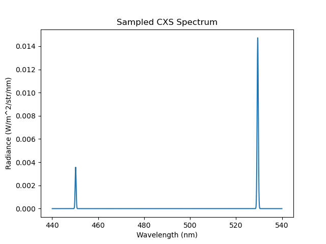
Caption: The observed spectrum reveals observations of both active charge exchange lines.

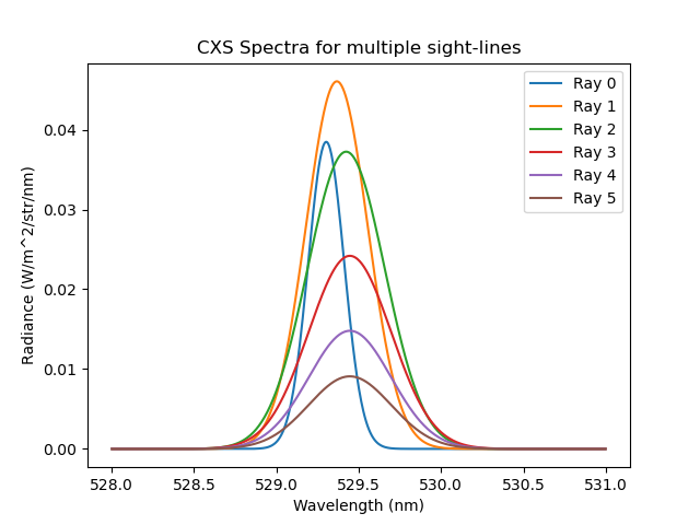
Caption: A zoomed in spectral view of the commonly studied CVI n = 8->7 CXS line. The lines are doppler shifted due to the velocity of the plasma.