Beam Emission Spectroscopy

This demonstration shows how to model the Beam Emission Spectrum (BES) from a beam-plasma interaction. These features are sometimes also known as the Motional Stark Effect (MSE) features. A slab plasma is setup as the target, with a neutral beam injected along the x axis. It is possible to change the sigma to pi ratios by overriding the line ratio functions as arguments to the BeamEmissionLine() model.

import numpy as np
import matplotlib.pyplot as plt

from raysect.optical import World, translate, rotate_basis, Vector3D, Point3D, Ray
from raysect.optical.observer import PinholeCamera

from cherab.core import Beam
from cherab.core.math import sample3d
from cherab.core.atomic import hydrogen, deuterium, carbon, Line
from cherab.core.model import SingleRayAttenuator, BeamEmissionLine, \
    ExcitationLine, RecombinationLine
from cherab.core.model.beam.beam_emission import SIGMA_TO_PI, SIGMA1_TO_SIGMA0, \
    PI2_TO_PI3, PI4_TO_PI3
from cherab.tools.plasmas.slab import build_slab_plasma
from cherab.openadas import OpenADAS


###############
# Make Plasma #

world = World()

plasma = build_slab_plasma(width=1.0, height=3.0, peak_density=1e18, neutral_temperature=20.0,
                           impurities=[(carbon, 6, 0.005)], parent=world)
plasma.b_field = Vector3D(0, 1.5, 0)
plasma.atomic_data = OpenADAS(permit_extrapolation=True)

# add background emission
h_alpha = Line(hydrogen, 0, (3, 2))
plasma.models = [ExcitationLine(h_alpha), RecombinationLine(h_alpha)]


####################
# Visualise Plasma #

h0 = plasma.composition.get(hydrogen, 0)
h1 = plasma.composition.get(hydrogen, 1)
c6 = plasma.composition.get(carbon, 6)

# Run some plots to check the distribution functions and emission profile are as expected
ti = h1.distribution.effective_temperature
r, _, z, t_samples = sample3d(ti, (-1, 2, 200), (0, 0, 1), (-1, 1, 200))
plt.imshow(np.transpose(np.squeeze(t_samples)), extent=[-1, 2, -1, 1])
plt.colorbar()
plt.axis('equal')
plt.xlabel('x axis')
plt.ylabel('z axis')
plt.title("Ion temperature profile in x-z plane")

plt.figure()
r, _, z, t_samples = sample3d(h0.distribution.density, (-1, 2, 200), (0, 0, 1), (-1, 1, 200))
plt.imshow(np.transpose(np.squeeze(t_samples)), extent=[-1, 2, -1, 1])
plt.colorbar()
plt.axis('equal')
plt.xlabel('x axis')
plt.ylabel('z axis')
plt.title("Neutral Density profile in x-z plane")


###########################
# Inject beam into plasma #

adas = OpenADAS(permit_extrapolation=True, missing_rates_return_null=True)

integration_step = 0.0025
beam_transform = translate(-0.5, 0.0, 0) * rotate_basis(Vector3D(1, 0, 0), Vector3D(0, 0, 1))

beam_energy = 110000  # keV
beam_current = 10  # A
beam_sigma = 0.05
beam_divergence = 1.3  # degree
beam_length = 3.0
beam_temperature = 1.0

bes_full_model = BeamEmissionLine(Line(deuterium, 0, (3, 2)),
                                  sigma_to_pi=SIGMA_TO_PI, sigma1_to_sigma0=SIGMA1_TO_SIGMA0,
                                  pi2_to_pi3=PI2_TO_PI3, pi4_to_pi3=PI4_TO_PI3)

beam_full = Beam(parent=world, transform=beam_transform)
beam_full.plasma = plasma
beam_full.atomic_data = adas
beam_full.energy = beam_energy
beam_full.power = 3e6  # beam_energy * beam_current
beam_full.temperature = beam_temperature
beam_full.element = deuterium
beam_full.sigma = beam_sigma
beam_full.divergence_x = beam_divergence
beam_full.divergence_y = beam_divergence
beam_full.length = beam_length
beam_full.attenuator = SingleRayAttenuator(clamp_to_zero=True)
beam_full.models = [bes_full_model]
beam_full.integrator.step = integration_step
beam_full.integrator.min_samples = 10

bes_half_model = BeamEmissionLine(Line(deuterium, 0, (3, 2)),
                                  sigma_to_pi=SIGMA_TO_PI, sigma1_to_sigma0=SIGMA1_TO_SIGMA0,
                                  pi2_to_pi3=PI2_TO_PI3, pi4_to_pi3=PI4_TO_PI3)

beam_half = Beam(parent=world, transform=beam_transform)
beam_half.plasma = plasma
beam_half.atomic_data = adas
beam_half.energy = beam_energy / 2
beam_half.power = 3e6  # beam_energy / 2 * beam_current
beam_half.temperature = beam_temperature
beam_half.element = deuterium
beam_half.sigma = beam_sigma
beam_half.divergence_x = beam_divergence
beam_half.divergence_y = beam_divergence
beam_half.length = beam_length
beam_half.attenuator = SingleRayAttenuator(clamp_to_zero=True)
beam_half.models = [bes_half_model]
beam_half.integrator.step = integration_step
beam_half.integrator.min_samples = 10

bes_third_model = BeamEmissionLine(Line(deuterium, 0, (3, 2)),
                                   sigma_to_pi=SIGMA_TO_PI, sigma1_to_sigma0=SIGMA1_TO_SIGMA0,
                                   pi2_to_pi3=PI2_TO_PI3, pi4_to_pi3=PI4_TO_PI3)

beam_third = Beam(parent=world, transform=beam_transform)
beam_third.plasma = plasma
beam_third.atomic_data = adas
beam_third.energy = beam_energy / 3
beam_third.power = 3e6  # beam_energy / 3 * beam_current
beam_third.temperature = beam_temperature
beam_third.element = deuterium
beam_third.sigma = beam_sigma
beam_third.divergence_x = beam_divergence
beam_third.divergence_y = beam_divergence
beam_third.length = beam_length
beam_third.attenuator = SingleRayAttenuator(clamp_to_zero=True)
beam_third.models = [bes_third_model]
beam_third.integrator.step = integration_step
beam_third.integrator.min_samples = 10


######################################
# Visualise beam behaviour in Plasma #

beam_density = np.empty((200, 200))
xpts = np.linspace(-1, 2, 200)
ypts = np.linspace(-1, 1, 200)
for i, xpt in enumerate(xpts):
    for j, ypt in enumerate(ypts):
        pt = Point3D(xpt, ypt, 0).transform(beam_full.to_local())
        beam_density[i, j] = beam_full.density(pt.x, pt.y, pt.z)

plt.ion()
plt.figure()
plt.imshow(np.transpose(beam_density), extent=[-1, 2, -1, 1], origin='lower')
los_start = Point3D(1.5, -1, 0)
los_target = Point3D(0.5, 0, 0)
los_direction = los_start.vector_to(los_target).normalise()
plt.plot([los_start.x, los_target.x], [los_start.y, los_target.y], 'k')
plt.xlim(-1, 2)
plt.ylim(-1, 1)
plt.colorbar()
plt.axis('equal')
plt.xlabel('x axis')
plt.ylabel('y axis')
plt.title("Beam full energy density profile in x-y plane")


z = np.linspace(0, 3, 200)
beam_full_densities = [beam_full.density(0, 0, zz) for zz in z]
beam_half_densities = [beam_half.density(0, 0, zz) for zz in z]
beam_third_densities = [beam_third.density(0, 0, zz) for zz in z]
plt.figure()
plt.plot(z, beam_full_densities, label="full energy")
plt.plot(z, beam_half_densities, label="half energy")
plt.plot(z, beam_third_densities, label="third energy")
plt.xlabel('z axis (beam coords)')
plt.ylabel('beam component density [m^-3]')
plt.title("Beam attenuation by energy component")
plt.legend()


ray = Ray(origin=Point3D(*los_start), direction=los_direction,
          min_wavelength=640, max_wavelength=670, bins=2000)
s = ray.trace(world)
plt.figure()
plt.plot(s.wavelengths, s.samples)
plt.xlabel('Wavelength (nm)')
plt.ylabel('Radiance (W/m^2/str/nm)')
plt.title('Sampled BES Spectrum')


transform = translate(1.25, -3.5, 0) * rotate_basis(Vector3D(0, 1, 0), Vector3D(0, 0, 1))
camera = PinholeCamera((128, 128), parent=world, transform=transform)
camera.spectral_rays = 1
camera.spectral_bins = 15
camera.pixel_samples = 50
camera.observe()
plt.ioff()
plt.show()

Caption: A camera view of a beam entering a slab plasma. The camera is tuned to D-alpha light. We can see the background passive emission of the neutrals hitting the slab as well as the beam emission light.

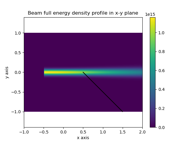
Caption: A x-z slice of the beam density profile showing the optical sightline. The amount of Motional Stark Effect (MSE) splitting is direction dependent.

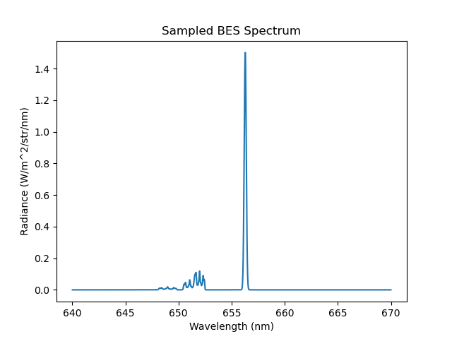
Caption: The full beam emission spectrum showing the passive emision peak as well as the three beam emission multiplet components.

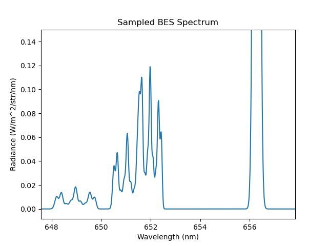
Caption: A zoomed in view of the BES feature.